
You are currently browsing the tag archive for the ‘statistics’ tag.
Some people were asked to name their favorite number, others were asked to give a random number:
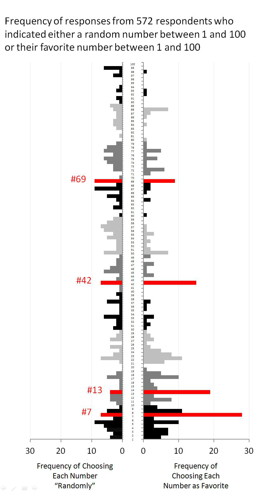
More here. Via Justin Wolfers.
Matthew Rabin was here last week presenting his work with Erik Eyster about social learning. The most memorable theme of their their papers is what they call “anti-imitation.” It’s the subtle incentive to do the opposite of someone in your social network even if you have the same preferences and there are no direct strategic effects.
You are probably familiar with the usual herding logic. People in your social network have private information about the relative payoff of various actions. You see their actions but not their information. If their action reveals they have strong information in favor of it you should copy them even if you have private information that suggests doing the opposite.
Most people who know this logic probably equate social learning with imitation and eventual herding. But Eyster and Rabin show that the same social learning logic very often prescribes doing the opposite of people in your social network. Here is a simple intuition. Start with a different, but simpler problem. Suppose that your friend makes an investment and his level of investment reveals how optimistic he is. His level of optimism is determined by two things, his prior belief and any private information he received.
You don’t care about his prior, it doesn’t convey any information that’s useful to you but you do want to know what information he got. The problem is the prior and the information are entangled together and just by observing his investment you can’t tease out whether he is optimistic because he was optimistic a priori or because he got some bullish information.
Notice that if somebody comes and tells you that his prior was very bullish this will lead you to downgrade your own level of optimism. Because holding his final beliefs fixed, the more optimistic was his prior the less optimistic must have been his new information and its that new information that matters for your beliefs. You want to do the opposite of his prior.
This is the basic force behind anti-imitation. (By the way I found it interesting that the English language doesn’t seem to have a handy non-prefixed word that means “doing the opposite of.”) Suppose now your friend got his prior beliefs from observing his friend. And now you see not only your friend’s investment level but his friend’s too. You have an incentive to do the opposite of his friend for exactly the same reason as above.
This assumes his friend’s action conveys no information of direct relevance for your own decision. And that leads to the prelim question. Consider a standard herding model where agents move in sequence first observing a private signal and then acting. But add the following twist. Each agent’s signal is relevant only for his action and the action of the very next agent in line. Agent 3 is like you in the example above. He wants to anti-imitate agent 1. But what about agents 4,5,6, etc?
You are walking back to your office in the rain and your path is lined by a row of trees. You could walk under the trees or you could walk in the open. Which will keep you drier?
If it just started raining you can stay dry by walking under the trees. On the other hand, when the rain stops you will be drier walking in the open. Because water will be falling off the leaves of the tree even though it has stopped raining. Indeed when the rain is tapering off you are better off out in the open. And when the rain is increasing you are better off under the tree.
What about in steady state? Suppose it has been raining steadily for some time, neither increasing nor tapering off. The rain that falls onto the top of the tree gets trapped by leaves. But the leaves can hold only so much water. When they reach capacity water begins to fall off the leaves onto you below. In equilibrium the rate at which water falls onto the top of the tree, which is the same rate it would fall on you if you were out in the open, equals the rate at which water falls off the leaves onto you.
Still you are not indifferent: you will stay drier out in the open. Under the tree the water that falls onto you, while constituting an equal total volume as the water that would hit you out in the open, is concentrated in larger drops. (The water pools as it sits on the leaves waiting to be pushed off onto you.) Your clothes will be dotted with fewer but larger water deposits and an equal volume of water spread over a smaller surface area will dry slower.
It is important in all this that you are walking along a line of trees and not just standing in one place. Because although the rain lands uniformly across the top of the tree, it is probably channeled outward away from the trunk as it falls from leaf to leaf and eventually below. (I have heard that this is true of Louisiana Oaks.) So the rainfall is uniform out in the open but not uniform under the tree. This means that no matter where you stand out in the open you will be equally wet, but there will be spots under the tree in which the rainfall will be greater than and less than that average. You can stand at the local minimum and be drier than you would out in the open.
Why are conditional probabilities so rarely used in court, and sometimes even prohibited? Here’s one more good reason: prosecution bias.
Suppose that a piece of evidence X is correlated with guilt. The prosecutor might say, “Conditional on evidence X, the likelihood ratio for guilt versus innoncence is Y, update your priors accordingly.” Even if the prosecutor is correct in his statistics his claim is dubious.
Because the prosecutor sees the evidence for all suspects before deciding which ones to bring to trial. And the jurors know this. So the fact that evidence like X exists against this defendant is already partially reflected in the fact that it was this guy they brought charges against and not someone else.
If jurors were truly Bayesian (a necessary presumption if we are to consider using probabiilties in court at all) then they would already have accounted for this and updated their priors accordingly before even learning that evidence X exists. When they are actually told it would necessarily move their priors less than what the statistics imply, perhaps hardly at all, maybe even in the opposite direction.
Why does it seem like the other queue is more often moving faster than yours? Here’s MindHacks:
So here we have a mechanism which might explain my queuing woes. The other lanes or queues moving faster is one salient event, and my intuition wrongly associates it with the most salient thing in my environment – me. What, after all, is more important to my world than me. Which brings me back to the universe-victim theory. When my lane is moving along I’m focusing on where I’m going, ignoring the traffic I’m overtaking. When my lane is stuck I’m thinking about me and my hard luck, looking at the other lane. No wonder the association between me and being overtaken sticks in memory more.
Which is one theory. But how about this theory: because it is in fact more often moving faster than yours. It’s true by definition because out of the total time in your life you spent in queues, the time spent in the slow queues is necessarily longer than the time spent in the fast queues.
Dear Northwestern Economics community. I was among the first to submit my bracket and I have already chosen all 16 teams seeded #1 through #4 to be eliminated in the first round of the NCAA tournament. In case you don’t believe me:

Now that i got that out of the way, consider the following complete information strategic-form game. Someone will throw a biased coin which comes up heads with probability 5/8. Two people simultaneously make guesses. A pot of money will be divided equally among those who correctly guessed how the coin would land. (Somebody else gets the money if both guess incorrectly.)
In a symmetric equilibrium of this game the two players will randomize their guesses in such a way that each earns the same expected payoff. But now suppose that player 1 can publicly announce his guess before player 2 moves. Player 1 will choose heads and player 2’s best reply is to choose tails. By making this announcement, player 1 has increased his payoff to a 5/8 chance of winning the pot of money.
This principle applies to just about any variety of bracket-picking game, hence my announcement. In fact in the psychotic version we play in our department, the twisted-brain child of Scott Ogawa, each matchup in the bracket is worth 1000 points to be divided among all who correctly guess the winner, and the overall winner is the one with the most points. Now that all of my colleagues know that the upsets enumerated above have already been taken by me their best responses are to pick the favorites and sure they will be correct with high probability on each, but they will split the 1000 points with everyone else and I will get the full 1000 on the inevitable one or two upsets that will come from that group.
The Walt Disney Co. recently announced its intention to “evolve” the experience of its theme park guests with the ultimate goal of giving everyone an RFID-enabled bracelet to transform their every move through the company’s parks and hotels into a steady stream of information for the company’s databases.
…Tracking the flow through the parks will come next. Right now, the park prints out pieces of paper called “FastPasses” to let people get reservations to ride. The wristbands and golden orbs will replace these slips of paper and most of everything else. Every reservation, every purchase, every ride on Dumbo, and maybe every step is waiting to be noticed, recorded, and stored away in a vast database. If you add up the movements and actions, it’s easy to imagine leaving a trail of hundreds of thousands of bytes of data after just one day in the park. That’s a rack of terabyte drives just to record this.
Theory question: Suppose Disney develops a more efficient rationing system than the current one with queues and then adjusts the price to enter the park optimally. In the end will your waiting time go up or down?
Eartip: Drew Conway
Comes from being able to infer that since by now you have not found any clear reason to favor one choice over the other it means that you are close to indifferent and you should pick now, even randomly.
It was the way he treated last-second, buzzer-beating three-pointers. Not close shots at the end of a game or shot clock, but half-courters at the end of each of the first three quarters. He seemed to be purposely letting the ball go just a half-second after the buzzer went off, presumably in order to shield his shooting percentage from the one-in-100 shot he was attempting. If the shot missed, no harm all around. If it went in? Then the crowd would go nuts and he’d get a few slaps on the back, even if he wouldn’t earn three points for the scoreboard.
In Baseball, a sacrifice is not scored as an at-bat and this alleviates somewhat the player/team conflict of interest. The coaches should lobby for a separate shooting category “buzzer-beater prayers.” As an aside, check out Kevin Durant’s analysis:
“It depends on what I’m shooting from the field. First quarter if I’m 4-for-4, I let it go. Third quarter if I’m like 10-for-16, or 10-for-17, I might let it go. But if I’m like 8-for-19, I’m going to go ahead and dribble one more second and let that buzzer go off and then throw it up there. So it depends on how the game’s going.”
This seems backward. 100% (4-4) is much bigger than 80% (4/5) whereas the difference between 8 for 19 and 8 for 20 is just 2 percentage points.

One reason people over-react to information is that they fail to recognize that the new information is redundant. If two friends tell you they’ve heard great things about a new restaurant in town it matters whether those are two independent sources of information or really just one. It may be that they both heard it from the same source, a recent restaurant review in the newspaper. When you neglect to account for redundancies in your information you become more confident in your beliefs than is justified.
This kind of problem gets worse and worse when the social network becomes more connected because its ever more likely that your two friends have mutual friends.
And it can explain an anomaly of psychology: polarization. Sandeep in his paper with Peter Klibanoff and Eran Hanany give a good example of polarization.
A number of voters are in a television studio before a U.S. Presidential debate. They are asked the likelihood that the Democratic candidate will cut the budget deficit, as he claims. Some think it is likely and others unlikely. The voters are asked the same question again after the debate. They become even more convinced that their initial inclination is correct.
It’s inconsistent with Bayesian information processing for groups who observe the same information to systematically move their beliefs in opposite directions. But polarization is not just the observation that the beliefs move in opposite directions. It’s that the information accentuates the original disagreement rather than reducing it. The groups move in the same opposite directions that caused their disagreement originally.
Here’s a simple explanation for it that as far as I know is a new one: the voters fail to recognize that the debate is not generating any new information relative to what they already knew.
Prior to the debate the voters had seen the candidate speaking and heard his view on the issue. Even if these voters had no bias ex ante, their differential reaction to this pre-debate information separates the voters into two groups according to whether they believe the candidate will cut the deficit or not.
Now when they see the debate they are seeing the same redundant information again. If they recognized that the information was redundant they would not move at all. But if don’t then they are all going to react to the debate in the same way they reacted to the original pre-debate information. Each will become more confident in his beliefs. As a result they will polarize even further.
Note that an implication of this theory is that whenever a common piece of information causes two people to revise their beliefs in opposite directions it must be to increase polarization, not reduce it.
I read this interesting post which talks about spectator sports and the gap between the excitement of watching in person versus on TV. The author ranks hockey as the sport with the largest gap: seeing hockey in person is way more fun than watching on TV. I think I agree with that and generally with the ranking given. (I would add one thing about American Football. With the advent of widescreen TVs the experience has improved a lot. But its still very dumb how they frame the shot to put the line of scrimmage down the center of the screen. The quarterback should be near the left edge of the screen at all times so that we can see who he is looking at downfield.)
But there was one off-hand comment that I think the author got completely wrong.
I think NBA basketball players might be the best at what they do in all of sports.
The thought experiment is to compare players across sports. I.e., are basketball players better at basketball than, say, snooker players are at playing snooker?
Unless you count being tall as one of the things NBA basketball players “do” I would say on the contrary that NBA basketball players must be among the worst at what they do in all of professional sports. The reason is simple: because height is so important in basketball, the NBA is drawing the top talent among a highly selected sub-population: those that are exceptionally tall. The skill distribution of the overall population, focusing on those skills that make a great basketball player like coordination, quickness, agility, accuracy; certainly dominate the distribution of the subpopulation from which the NBA draws its players.
Imagine that the basket was lowered by 1 foot and a height cap enforced so that in order to be eligible to play you must be 1 foot shorter than the current tallest NBA player (or you could scale proportionally if you prefer.) The best players in that league would be better at what they do than current NBA players. (Of course you need to allow equilibrium to be reached where young players currently too short to be NBA stars now make/receive the investments and training that the current elite do.)
Now you might ask why we should discard height as one of the bundle of attributes that we should say a player is “best” at. Aren’t speed, accuracy, etc. all talents that some people are born with and others are not, just like height? Definitely so, but ask yourself this question. If a guy stops playing basketball for a few years and then takes it up again, which of these attributes is he going to fall the farthest behind the cohort who continued to train uninterrupted? He’ll probably be a step slower and have lost a few points in shooting percentage. He won’t be any shorter than he would have been.
When you look at a competition where one of the inputs of the production function is an exogenously distributed characteristic, players with a high endowment on that dimension have a head start. This has two effects on the distribution of the (partially) acquired characteristics that enter the production function. First, there is the pure statistical effect I alluded to above. If success requires some minimum height then the pool of competitors excludes a large component of the population.
There is a second effect on endogenous acquisition of skills. Competition is less intense and they have less incentive to acquire skills in order to be competitive. So even current NBA players are less talented than they would be if competition was less exclusive.
So what are the sports whose athletes are the best at what they do? My ranking
- Table Tennis
- Soccer
- Tennis
- Golf
- Chess
Suppose that what makes a person happy is when their fortunes exceed expectations by a discrete amount (and that falling short of expectations is what makes you unhappy.) Then simply because of convergence of expectations:
- People will have few really happy phases in their lives.
- Indeed even if you lived forever you would have only finitely many spells of happiness.
- Most of the happy moments will come when you are young.
- Happiness will be short-lived.
- The biggest cross-sectional variance in happiness will be among the young.
- When expectations adjust to the rate at which your fortunes improve, chasing further happiness requires improving your fortunes at an accelerating rate.
- If life expectancy is increasing and we simply extrapolate expectations into later stages of life we are likely to be increasingly depressed when we are old.
- There could easily be an inverse relationship between intelligence and happiness.
The average voter’s prior belief is that the incumbent is better than the challenger. Because without knowing anything more about either candidate, you know that the incumbent defeated a previous opponent. To the extent that the previous electoral outcome was based on the voters’ information about the candidates this is good news about the current incumbent. No such inference can be made about the challenger.
Headline events that occurred during the current incumbent’s term were likely to generate additional information about the incumbent’s fitness for office. The bigger the headline the more correlated that information is going to be among the voters. For example, a significant natural disaster such as Hurricane Katrina or Hurricane Sandy is likely to have a large common effect on how voters’ evaluate the incumbent’s ability to manage a crisis.
For exactly this reason, an event like that is bad for the incumbent on average. Because the incumbent begins with the advantage of the prior. The upside benefit of a good signal is therefore much smaller than the downside risk of a bad signal.
As I understand it, this is the theory developed in a paper by Ethan Bueno de Mesquita and Scott Ashworth, who use it to explain how events outside of the control of political leaders (like natural disasters) seem, empirically, to be blamed on incumbents. This pattern emerges in their model not because voters are confused about political accountability, but instead through the informational channel outlined above.
It occurs to me that such a model also explains the benefit of saturation advertising. The incumbent unleashes a barrage of ads to drive voters away from their televisions thus cutting them off from information and blunting the associated risks. Note that after the first Obama-Romney debate, Obama’s national poll numbers went south but they held steady in most of the battleground states where voters had already been subjected to weeks of wall-to-wall advertising.
Tyler Cowen and Kevin Grier mention a curious fact:
Economists Andrew Healy, Neil Malhotra, and Cecilia Mo make this argument in afascinating article in the Proceedings of the National Academy of Science. They examined whether the outcomes of college football games on the eve of elections for presidents, senators, and governors affected the choices voters made. They found that a win by the local team, in the week before an election, raises the vote going to the incumbent by around 1.5 percentage points. When it comes to the 20 highest attendance teams—big athletic programs like the University of Michigan, Oklahoma, and Southern Cal—a victory on the eve of an election pushes the vote for the incumbent up by 3 percentage points. That’s a lot of votes, certainly more than the margin of victory in a tight race. And these results aren’t based on just a handful of games or political seasons; the data were taken from 62 big-time college teams from 1964 to 2008.
And Andrew Gelman signs off on it.
I took a look at the study (I felt obliged to, as it combined two of my interests) and it seemed reasonable to me. There certainly could be some big selection bias going on that the authors (and I) didn’t think of, but I saw no obvious problems. So for now I’ll take their result at face value and will assume a 2 percentage-point effect. I’ll assume that this would be +1% for the incumbent party and -1% for the other party, I assume.
Let’s try this:
- Incumbents have an advantage on average.
- Higher overall turnout therefore implies a bigger margin for the incumbent, again on average.
- In sports, the home team has an advantage on average.
- Conditions that increase overall scoring amplify the advantage of the home team.
- Good weather increases overall turnout in an election and overall scoring in a football game.
So what looks like football causes elections could really be just good weather causes both. Note well, I have not actually read the paper but I did search for the word weather and it appears nowhere.
From Nature news.
Calcagno, in contrast, found that 3–6 years after publication, papers published on their second try are more highly cited on average than first-time papers in the same journal — regardless of whether the resubmissions moved to journals with higher or lower impact.
Calcagno and colleagues think that this reflects the influence of peer review: the input from referees and editors makes papers better, even if they get rejected at first.
Based on my experience with economics journals as an editor and author I highly doubt that. Authors pay very close attention to referees’ demands when they are asked to resubmit to the same journal because of course those same referees are going to decide on the next round. On the other hand authors pretty much ignore the advice of referees who have proven their incompetence by rejecting their paper.
Instead my hypothesis is that authors with good papers start at the top journals and expect a rejection or two (on average) before the paper finally lands somewhere reasonably good. Authors of bad papers submit them to bad journals and have them accepted right away. Drew Fudenberg suggested something similar.
Its the same reason the lane going in the opposite direction is always flowing faster. This is a lovely article that works through the logic of conditional proportions. I really admire this kind of lucid writing about subtle ideas. (link fixed now, sorry.)
This phenomenon has been called the friendship paradox. Its explanation hinges on a numerical pattern — a particular kind of “weighted average” — that comes up in many other situations. Understanding that pattern will help you feel better about some of life’s little annoyances.
For example, imagine going to the gym. When you look around, does it seem that just about everybody there is in better shape than you are? Well, you’re probably right. But that’s inevitable and nothing to feel ashamed of. If you’re an average gym member, that’s exactly what you should expect to see, because the people sweating and grunting around you are not average. They’re the types who spend time at the gym, which is why you’re seeing them there in the first place. The couch potatoes are snoozing at home where you can’t count them. In other words, your sample of the gym’s membership is not representative. It’s biased toward gym rats.
Nate Silver’s 538 Election Forecast has consistently given Obama a higher re-election probability than InTrade does. The 538 forecast is based on estimating vote probabilities from State polls and simulating the Electoral College. InTrade is just a betting market where Obama’s re-election probability is equated with the market price of a security that pays off $1 in the event that Obama wins. How can we decide which is the more accurate forecast? When you log on in the morning and see that InTrade has Obama at 70% and Nate Silver has him at 80%, on what basis can we say that one of them is right and the other is wrong?
At a philosophical level we can say they are both wrong. Either Obama is going to win or Romney is going to win so the only correct forecast would give one of them 100% chance of winning. Slightly less philosophically, is there any interpretation of the concept of “probability” relative to which we can judge these two forecasting methods?
One way is to define probability simply as the odds at which you would be indifferent between betting one way or the other. InTrade is meant to be the ideal forecast according to this interpretation because of course you can actually go and bet there. If you are not there betting right now then we can infer you agree with the odds. One reason among many to be unsatisfied with this conclusion is that there are many other betting sites where the odds are dramatically different.
Then there’s the Frequentist interpretation. Based on all the information we have (especially polls) if this situation were repeated in a series of similar elections, what fraction of those elections would eventually come out in Obama’s favor? Nate Silver is trying to do something like this. But there is never going to be anything close to enough data to be able to test whether his model is getting the right frequency.
Nevertheless, there is a way to assess any forecasting method that doesn’t require you to buy into any particular interpretation of probability. Because however you interpret it, mathematically a probability estimate has to satisfy some basic laws. For a process like an election where information arrives over time about an event to be resolved later, one of these laws is called the Martingale property.
The Martingale property says this. Suppose you checked the forecast in the morning and it said Obama 70%. And then you sit down to check the updated forecast in the evening. Before you check you don’t know exactly how its going to be revised. Sometimes it gets revised upward, sometimes downard. Soometimes by a lot, sometimes just a little. But if the forecast is truly a probability then on average it doesn’t change at all. Statistically we should see that the average forecast in the evening equals the actual forecast in the morning.
We can be pretty confident that Nate Silver’s 538 forecast would fail this test. That’s because of how it works. It looks at polls and estimates vote shares based on that information. It is an entirely backward-looking model. If there are any trends in the polls that are discernible from data these trends will systematically reflect themselves in the daily forecast and that would violate the Martingale property. (There is some trendline adjustment but this is used to adjust older polls to estimate current standing. And there is some forward looking adjustment but this focuses on undecided voters and is based on general trends. The full methodology is described here.)
In order to avoid this problem, Nate Silver would have to do the following. Each day prior to the election his model should forecast what the model is going to say tomorrow, based on all of the available information today (think about that for a moment.) He is surely not doing that.
So 70% is not a probability no matter how you prefer to interpret that word. What does it mean then? Mechanically speaking its the number that comes out of a formula that combines a large body of recent polling data in complicated ways. It is probably monotonic in the sense that when the average poll is more favorable for Obama then a higher number comes out. That makes it a useful summary statistic. It means that if today his number is 70% and yesterday it was 69% you can logically conclude that his polls have gotten better in some aggregate sense.
But to really make the point about the difference between a simple barometer like that and a true probability, imagine taking Nate Silver’s forecast, writing it as a decimal (70% = 0.7) and then squaring it. You still get a “percentage,” but its a completely different number. Still its a perfectly valid barometer: its monotonic. By contrast, for a probability the actual number has meaning beyond the fact that it goes up or down.
What about InTrade? Well, if the market it efficient then it must be a Martingale. If not, then it would be possible to predict the day-to-day drift in the share price and earn arbitrage profits. On the other hand the market is clearly not efficient because the profits from arbitraging the different prices at BetFair and InTrade have been sitting there on the table for weeks.
In a meeting a guy’s phone goes off because he just received a text and he forgot to silence it. What kind of guy is he?
- He’s the type who is a slave to his smartphone, constantly texting and receiving texts. Statistically this must be true because conditional on someone receiving a text it is most likely the guy whose arrival rate of texts is the highest.
- He’s the type who rarely uses his phone for texting and this is the first text he has received in weeks. Statistically this must be true because conditional on someone forgetting to silence his phone it is most likely the guy whose arrival rate of texts is the lowest.

My 9 year-old daughter’s soccer games are often high-scoring affairs. Double-digit goal totals are not uncommon. So when her team went ahead 2-0 on Saturday someone on the sideline remarked that 2-0 is not the comfortable lead that you usually think it is in soccer.
But that got me thinking. Its more subtle than that. Suppose that the game is 2 minutes old and the score is 2-0. If these were professional teams you would say that 2-0 is a good lead but there are still 88 minutes to play and there is a decent chance that a 2-0 lead can be overcome.
But if these are 9 year old girls and you know only that the score is 2-0 after 2 minutes your most compelling inference is that there must be a huge difference in the quality of these two teams and the team that is leading 2-0 is very likely to be ahead 20-0 by the time the game is over.
The point is that competition at higher levels is different in two ways. First there is less scoring overall which tends to make a 2-0 lead more secure. But second there is also lower variance in team quality. So a 2-0 lead tells you less about the matchup than it does at lower levels.
Ok so a 2-0 lead is a more secure lead for 9 year olds when 95% of the game remains to be played (they play for 40 minutes). But when 5% of the game remains to be played a 2-0 lead is almost insurmountable at the professional level but can easily be upset in a game among 10 year olds.
So where is the flipping point? How much of the game must elapse so that a 2-0 lead leads to exactly the same conditional probability that the 9 year olds hold on to the lead and win as the professionals?
Next question. Let F be the fraction of the game remaining where the 2-0 lead flipping point occurs. Now suppose we have a 3-0 lead with F remaining. Who has the advantage now?
And of course we want to define F(k) to be the flipping point of a k-nil lead and we want to take the infinity-nil limit to find the flipping point F(infinity). Does it converge to zero or one, or does it stay in the interior?
Act as if you have log utility and with probability 1 your wealth will converge to infinity.
Sergiu Hart presented this paper at Northwestern last week. Suppose you are going to be presented an infinite sequence of gambles. Each has positive expected return but also a positive probability of a loss. You have to decide which gambles to accept and which gambles to reject. You can also invest purchase fractions of gambles: exposing yourself to some share 
Here is a simple investment strategy that guarantees infinite wealth. First, for every gamble 

Next, when your wealth level is actually 


If you follow this rule then no matter what sequence of gambles appears you will never go bankrupt and your wealth will converge to infinity. What’s more, this is in some sense the most aggressive investment strategy you can take without running the risk of going bankrupt. Foster and Hart show that any investor that is willing to accept some gambles


In basketball the team benches are near the baskets on opposite sides of the half court line. The coaches roam their respective halves of the court shouting directions to their team.
As in other sports the teams switch sides at halftime but the benches stay where they were. That means that for half of the game the coaches are directing their defenses and for the other half they are directing their offenses.
If coaching helps then we should see more scoring in the half where the offenses are receiving direction.
This could easily be tested.
Here is an excellent rundown of some soul searching in the neuroscience community regarding statistical significance. The standard method of analyzing brain scan data apparently involves something akin to data mining but the significance tests use standard single-hypothesis p-values.
One historical fudge was to keep to uncorrected thresholds, but instead of a threshold of p=0.05 (or 1 in 20) for each voxel, you use p=0.001 (or 1 in a 1000). This is still in relatively common use today, but it has been shown, many times, to be an invalid attempt at solving the problem of just how many tests are run on each brain-scan. Poldrack himself recently highlighted this issue by showing a beautiful relationship between a brain region and some variable using this threshold, even though the variable was entirely made up. In a hilarious earlier version of the same point, Craig Bennett and colleagues fMRI scanned a dead salmon, with a task involving the detection of the emotional state of a series of photos of people. Using the same standard uncorrected threshold, they found two clusters of activation in the deceased fish’s nervous system, though, like the Poldrack simulation, proper corrected thresholds showed no such activations.
Biretta blast: Marginal Revolution.
So there was this famous experiment and just recently a new team of researchers tried to replicate it and they could not. Quoting Alex Tabarrok:
You will probably not be surprised to learn that the new paper fails to replicate the priming effect. As we know from Why Most Published Research Findings are False (also here), failure to replicate is common, especially when sample sizes are small.
There’s a lot more at the MR link you should check it out. But here’s the thing. If most published research findings are false then which one is the false one, the original or the failed replication? Have you noticed that whenever a failed replication is reported, it is reported with all of the faith and fanfare that the original, now apparently disproven study was afforded? All we know is that one of them is wrong, can we really be sure which?
If I have to decide which to believe in, my money’s on the original. Think publication bias and ask yourself which is likely to be larger: the number of unpublished experiments that confirmed the original result or the number of unpublished results that didn’t.
Here’s a model. Experimenters are conducting a hidden search for results and they publish as soon as they have a good one. For the original experimenter a good result means a positive result. They try experiment A and it fails so they conclude that A is a dead end, shelve it and turn to something new, experiment B. They continue until they hit on a positive result, experiment X and publish it.
Given the infinity of possible original experiments they could try, it is very likely that when they come to experiment X they were the first team to ever try it. By contrast, Team-Non-Replicate searches among experiments that have already been published, especially the most famous ones. And for them a good result is a failure to replicate. That’s what’s going to get headlines.
Since X is a famous experiment it’s not going to take long before they try that. They will do a pilot experiment and see if they can fail to replicate it. If they fail to fail to replicate it, they are going to shelve it and go on to the next famous experiment. But then some other Team-Non-Replicate, who has no way of knowing this is a dead-end, is going to try experiment X, etc. This is going to continue until someone succeeds in failing to replicate.
When that’s all over let’s count the number of times X failed: 1. The number of times X was confirmed equals 1 plus the number of non-non-replications before the final successful failure.
Email is the superior form of communication as I have argued a few times before, but it can sure aggravate your self-control problems. I am here to help you with that.
As you sit in your office working, reading, etc., the random email arrival process is ticking along inside your computer. As time passes it becomes more and more likely that there is email waiting for you and if you can’t resist the temptation you are going to waste a lot of time checking to see what’s in your inbox. And it’s not just the time spent checking because once you set down your book and start checking you won’t be able to stop yourself from browsing the web a little, checking twitter, auto-googling, maybe even sending out an email which will eventually be replied to thereby sealing your fate for the next round of checking.
One thing you can do is activate your audible email notification so that whenever an email arrives you will be immediately alerted. Now I hear you saying “the problem is my constantly checking email, how in the world am i going to solve that by setting up a system that tells me when email arrives? Without the notification system at least I have some chance of resisting the temptation because I never know for sure that an email is waiting.”
Yes, but it cuts two ways. When the notification system is activated you are immediately informed when an email arrives and you are correct that such information is going to overwhelm your resistance and you will wind up checking. But, what you get in return is knowing for certain when there is no email waiting for you.
It’s a very interesting tradeoff and one we can precisely characterize with a little mathematics. But before we go into it, I want you to ask yourself a question and note the answer before reading on. On a typical day if you are deciding whether to check your inbox, suppose that the probability is p that you have new mail. What p is going to get you to get up and check? We know that you’re going to check if p=1 (indeed that’s what your mailbeep does, it puts you at p=1.) And we know that you are not going to check when p=0. What I want to know is what is the threshold above which its sufficiently likely that you will check and below which is sufficiently unlikely so you’ll keep on reading? Important: I am not asking you what policy you would ideally stick to if you could control your temptation, I am asking you to be honest about your willpower.
Ok, now that you’ve got your answer let’s figure out whether you should use your mailbeep or not. The first thing to note is that the mail arrival process is a Poisson process: the probability that an email arrives in a given time interval is a function only of the length of time, and it is determined by the arrival rate parameter r. If you receive a lot of email you have a large r, if the average time spent between arrivals is longer you have a small r. In a Poisson process, the elapsed time before the next email arrives is a random variable and it is governed by the exponential distribution.
Let’s think about what will happen if you turn on your mail notifier. Then whenever there is silence you know for sure there is no email, p=0 and you can comfortably go on working temptation free. This state of affairs is going to continue until the first beep at which point you know for sure you have mail (p=1) and you will check it. This is a random amount of time, but one way to measure how much time you waste with the notifier on is to ask how much time on average will you be able to remain working before the next time you check. And the answer to that is the expected duration of the exponential waiting time of the Poisson process. It has a simple expression:
Expected time between checks with notifier on =

Now let’s analyze your behavior when the notifier is turned off. Things are very different now. You are never going to know for sure whether you have mail but as more and more time passes you are going to become increasingly confident that some mail is waiting, and therefore increasingly tempted to check. So, instead of p lingering at 0 for a spell before jumping up to 1 now it’s going to begin at 0 starting from the very last moment you previously checked but then steadily and continuously rise over time converging to, but never actually equaling 1. The exponential distribution gives the following formula for the probability at time T that a new email has arrived.
Probability that email arrives at or before a given time T =

Now I asked you what is the p* above which you cannot resist the temptation to check email. When you have your notifier turned off and you are sitting there reading, p will be gradually rising up to the point where it exceeds p* and right at that instant you will check. Unlike with the notification system this is a deterministic length of time, and we can use the above formula to solve for the deterministic time T at which you succumb to temptation. It’s given by
Time between checks when the notifier is off =

And when we compare the two waiting times we see that, perhaps surprisingly, the comparison does not depend on your arrival rate r (it appears in the numerator of both expressions so it will cancel out when we compare them.) That’s why I didn’t ask you that, it won’t affect my prescription (although if you receive as much email as I do, you have to factor in that the mail beep turns into a Geiger counter and that may or may not be desirable for other reasons.) All that matters is your p* and by equating the two waiting times we can solve for the crucial cutoff value that determines whether you should use the beeper or not.
The beep increases your productivity iff your p* is smaller than

This is about .63 so if your p* is less than .63 meaning that your temptation is so strong that you cannot resist checking any time you think that there is at least a 63% chance there is new mail waiting for you then you should turn on your new mail alert. If you are less prone to temptation then yes you should silence it. This is life-changing advice and you are welcome.
Now, for the vapor mill and feeling free to profit, we do not content ourselves with these two extreme mechanisms. We can theorize what the optimal notification system would be. It’s very counterintuitive to think that you could somehow “trick” yourself into waiting longer for email but in fact even though you are the perfectly-rational-despite-being-highly-prone-to-temptation person that you are, you can. I give one simple mechanism, and some open questions below the fold.
It’s the canonical example of reference-dependent happiness. Someone from the Midwest imagines how much happier he would be in California but when he finally has the chance to move there he finds that he is just as miserable as he was before.
But can it be explained by a simple selection effect? Suppose that everyone who lives in the Midwest gets a noisy but unbiased signal of how happy they would be in California. Some overestimate how happy they would be and some underestimate it. Then they get random opportunities to move. Who is going to take that opportunity? Those who overestimate how happy they will be. And so when they arrive they are disappointed.
It also explains why people who are forced to leave California, say for job-related reasons, are pleasantly surprised at how happy they can be in the Midwest. Since they hadn’t moved voluntarily already, its likely that they underestimated how happy they would be.
These must be special cases of this paper by Eric van den Steen, and its similar to the logic behind Lazear’s theory behind the Peter Principle. (For the latter link I thank Adriana Lleras-Muney.)
In many situations, such reinforcement learning is an essential strategy, allowing people to optimize behavior to fit a constantly changing situation. However, the Israeli scientists discovered that it was a terrible approach in basketball, as learning and performance are “anticorrelated.” In other words, players who have just made a three-point shot are much more likely to take another one, but much less likely to make it:
What is the effect of the change in behaviour on players’ performance? Intuitively, increasing the frequency of attempting a 3pt after made 3pts and decreasing it after missed 3pts makes sense if a made/missed 3pts predicted a higher/lower 3pt percentage on the next 3pt attempt. Surprizingly [sic], our data show that the opposite is true. The 3pt percentage immediately after a made 3pt was 6% lower than after a missed 3pt. Moreover, the difference between 3pt percentages following a streak of made 3pts and a streak of missed 3pts increased with the length of the streak. These results indicate that the outcomes of consecutive 3pts are anticorrelated.
This anticorrelation works in both directions. as players who missed a previous three-pointer were more likely to score on their next attempt. A brick was a blessing in disguise.
The underlying study, showing a “failure of reinforcement learning” is here.
Suppose you just hit a 3-pointer and now you are holding the ball on the next possession. You are an experienced player (they used NBA data), so you know if you are truly on a hot streak or if that last make was just a fluke. The defense doesn’t. What the defense does know is that you just made that last 3-pointer and therefore you are more likely to be on a hot streak and hence more likely than average to make the next 3-pointer if you take it. Likewise, if you had just missed the last one, you are less likely to be on a hot streak, but again only you would know for sure. Even when you are feeling it you might still miss a few.
That means that the defense guards against the three-pointer more when you just made one than when you didn’t. Now, back to you. You are only going to shoot the three pointer again if you are really feeling it. That’s correlated with the success of your last shot, but not perfectly. Thus, the data will show the autocorrelation in your 3-point shooting.
Furthermore, when the defense is defending the three-pointer you are less likely to make it, other things equal. Since the defense is correlated with your last shot, your likelihood of making the 3-pointer is also correlated with your last shot. But inversely this time: if you made the last shot the defense is more aggressive so conditional on truly being on a hot streak and therefore taking the next shot, you are less likely to make it.
(Let me make the comparison perfectly clear: you take the next shot if you know you are hot, but the defense defends it only if you made the last shot. So conditional on taking the next shot you are more likely to make it when the defense is not guarding against it, i.e. when you missed the last one.)
You shoot more often and miss more often conditional on a previous make. Your private information about your make probability coupled with the strategic behavior of the defense removes the paradox. It’s not possible to “arbitrage” away this wedge because whether or not you are “feeling it” is exogenous.
I write all the time about strategic behavior in athletic competitions. A racer who is behind can be expected to ease off and conserve on effort since effort is less likely to pay off at the margin. Hence so will the racer who is ahead, etc. There is evidence that professional golfers exhibit such strategic behavior, this is the Tiger Woods effect.
We may wonder whether other animals are as strategically sophisticated as we are. There have been experiments in which monkeys play simple games of strategy against one another, but since we are not even sure humans can figure those out, that doesn’t seem to be the best place to start looking.
I would like to compare how humans and other animals behave in a pure physical contest like a race. Suppose the animals are conditioned to believe that they will get a reward if and only if they win a race. Will they run at maximum speed throughout regardless of their position along the way? Of course “maximum speed” is hard to define, but a simple test is whether the animal’s speed at a given point in the race is independent of whether they are ahead or behind and by how much.
And if the animals learn that one of them is especially fast, do they ease off when racing against her? Do the animals exhibit a tiger Woods effect?
There are of course horse-racing data. That’s not ideal because the jockey is human. Still there’s something we can learn from horse racing. The jockey does not internalize 100% of the cost of the horse’s effort. Thus there should be less strategic behavior in horse racing than in races between humans or between jockey-less animals. Dog racing? Does that actually exist?
And what if a dog races against a human, what happens then?
In the past few weeks Romney has dropped from 70% to under 50% and Gingrich has rocketed to 40% on the prediction markets. And in this time Obama for President has barely budged from its 50% perch. As someone pointed out on Twitter (I forget who, sorry) this is hard to understand.
For example if you think that in this time there has been no change in the conditional probabilities that either Gingrich or Romney beats Obama in the general election, then these numbers imply that the market thinks that those conditional probabilities are the same. Conversely, If you think that Gingrich has risen because his perceived odds of beating Obama have risen over the same period, then it must be that Romney’s have dropped in precisely the proportion to keep the total probability of a GOP president constant.
It’s hard to think of any public information that could have these perfectly offsetting effects. Here’s the only theory I could come up with that is consistent with the data. No matter who the Republican candidate is, he has a 50% chance of beating Obama. This is just a Downsian prediction. The GOP machine will move whoever it is to a median point in the policy space. But, and here’s the model, this doesn’t imply that the GOP is indifferent between Gingrich and Romney.
While any candidate, no matter what his baggage, can be repositioned to the Downsian sweet spot, the cost of that repositioning depends on the candidate, the opposition, and the political climate. The swing from Romney to Gingrich reflects new information about these that alters the relative cost of marketing the two candidates. Gingrich has for some reason gotten relatively cheaper.
I didn’t say it was a good theory.
Update: Rajiv Sethi reminded me that the tweet was from Richard Thaler. (And see Rajiv’s comment below.)
Stefan Lauermann points me to a new paper, this is from the abstract:
Our analysis shows that both stake size and communication have a significant impact on the player’s likelihood to cooperate. In particular, we observe a negative correlation between stake size and cooperation. Also certain gestures, as handshakes, decrease the likelihood to cooperate. But, if players mutually promise each other to cooperate and in addition shake hands on it, the cooperation rate increases.
Measuring social influence is notoriously difficult in observational data. If I like Tin Hat Trio and so do my friends is it because I influenced them or we just have similar tastes, as friends often do. A controlled experiment is called for. It’s hard to figure out how to do that. How can an experimenter cause a subject to like something new and then study the effect on his friends?
Online social networks open up new possibilities. And here is the first experiment I came across that uses Facebook to study social influence, by Johan Egebark and Mathias Ekstrom. If one of your friends “likes” an item on Facebook, will it make you like it too?
Making use of five Swedish users’ actual accounts, we create 44 updates in total during a seven month period.1 For every new update, we randomly assign our user’s friends into either a treatment or a control group; hence, while both groups are exposed to identical status updates, treated individuals see the update after someone (controlled by us) has Liked it whereas individuals in the control group see it without anyone doing so. We separate between three different treatment conditions: (i) one unknown user Likes the update, (ii) three unknown users Like the update and (iii) one peer Likes the update. Our motivation for altering treatments is that it enables us to study whether the number of previous opinions as well as social proximity matters.2 The result from this exercise is striking: whereas the first treatment condition left subjects unaffected, both the second and the third more than doubled the probability of Liking an update, and these effects are statistically significant.
