
You are currently browsing the tag archive for the ‘statistics’ tag.
I was working on a paper, writing the introduction to a new section that deals with an extension of the basic model. It’s a relevant extension because it fits many real-world applications. So naturally I started to list the many real-world applications.
“This applies to X, Y, and….” hmmm… what’s the Z? Nothing coming to mind.
But I can’t just stop with X and Y. Two examples are not enough. If I only list two examples then the reader will know that I could only think of two examples and my pretense that this extension applies to many real-world applications will be dead on arrival.
I really only need one more. Because if I write “This applies to X, Y, Z, etc.” then the Z plus the “etc.” proves that there is in fact a whole blimpload of examples that I could have listed and I just gave the first three that came to mind, then threw in the etc. to save space.
If you have ever written anything at all you know this feeling. Three equals infinity but two is just barely two.
This is largely an equilbrium phenomenon. A convention emerged according to which those who have an abundance of examples are required to prove it simply by listing three. Therefore those who have listed only two examples truly must have only two.
Three isn’t the only threshold that would work as an equilibrium. There are many possibilities such as two, four, five etc. (ha!) Whatever threshold N we settle on, authors will spend the effort to find N examples (if they can) and anything short of that will show that they cannot.
But despite the multiplicity I bet that the threshold of three did not emerge arbitrarily. Here is an experiment that illustrates what I am thinking.
Subjects are given a category and 1 minute, say. You ask them to come up with as many examples from that category they can think of in 1 minute. After the 1 minute is up and you count how many examples they came up with you then give them another 15 minutes to come up with as many as they can.
With these data we would do the following. Plot on the horizontal axis the number x of items they listed in the first minute and on the vertical axis the number E(y|x) equal to the empirical average number y of items they came up with in total conditional on having come up with x items in the first minute.
I predict that you will see an anomalous jump upwards between E(y|2) and E(y|3).
This experiment does not take into account the incentive effects that come from the threshold. The incentives are simply to come up with as many examples as possible. That is intentional. The point is that this raw statistical relation (if it holds up) is the seed for the equilibrium selection. That is, when authors are not being strategic, then three-or-more equals many more than two. Given that, the strategic response is to shoot for exactly three. The equilibrium result is that three equals infinity.
via Arthur Robson:
While appeals often unmask shaky evidence, this was different. This time, a mathematical formula was thrown out of court. The footwear expert made what the judge believed were poor calculations about the likelihood of the match, compounded by a bad explanation of how he reached his opinion. The conviction was quashed.
And the judge ruled that Bayes’ law for conditional probabilities could not be used in court. Statisticians, Mathematicians, and prosecutors are worried that justice will suffer as a result. The statistical evidence centered around the likelihood of a coincidental match of shoeprint with shoes owned by the Defendant.
In the shoeprint murder case, for example, it meant figuring out the chance that the print at the crime scene came from the same pair of Nike trainers as those found at the suspect’s house, given how common those kinds of shoes are, the size of the shoe, how the sole had been worn down and any damage to it. Between 1996 and 2006, for example, Nike distributed 786,000 pairs of trainers. This might suggest a match doesn’t mean very much. But if you take into account that there are 1,200 different sole patterns of Nike trainers and around 42 million pairs of sports shoes sold every year, a matching pair becomes more significant.
Now if I can prove to jurors that there was one shoe in the basement and another shoe upstairs, then probably I can legitimately claim to have proven that the total number of shoes is two because the laws of arithmetic should be binding on the jurors deductions. And if there is a chance that a juror comes to some different conclusion then it would make sense for an expert witness, or the judge even, tell the juror that he is making a mistake. Indeed a courtroom demonstration could prove the juror wrong.
But do the “laws” of probability have the same status? If I can prove to the juror that his prior should attach probability p to A and probability q to [A and B], and if the evidence proves that A is true, should he then be required to attach probability q/p to B? Suppose for example that a juror disagreed with this conclusion. Could he be proven wrong? A courtroom demonstration could show something about relative frequencies, but the juror could dispute that these have anything to do with probabilities.
It appears though that the judge’s ruling in this case was not on the basis of bayesian/frequentist philosophy, but rather about the validity of a Bayesian prescription when the prior itself is subjective.
The judge complained that he couldn’t say exactly how many of one particular type of Nike trainer there are in the country. National sales figures for sports shoes are just rough estimates.
And so he decided that Bayes’ theorem shouldn’t again be used unless the underlying statistics are “firm”. The decision could affect drug traces and fibre-matching from clothes, as well as footwear evidence, although not DNA.
This is a reasonable judgment even if the court upholds Bayesian logic per se. Because the prior probability of a second pair of matching shoes can be deduced from the sales figures only under some assumptions about the distribution of shoes with various tread patterns. The expert witnesses probably assumed that the accused and a hypothetical third-party murderer were randomly assigned tread patterns on their Nikes and that these assignments were independent. But if the two live in the same town and shop at the same shoe store and if that store sold shoes with the same tread pattern, then that assumption would significantly understate the probability of a match.

Let’s say I want to know how many students in my class are cheating on exams. Maybe I’d like to know who the individual cheaters are, maybe I don’t but let’s say that the only way I can find out the number of cheaters is to ask the students themselves to report whether or not they cheated. I have a problem because no matter how hard I try to convince them otherwise, they will assume that a confession will get them in trouble.
Since I cannot persuade them of my incentives, instead I need to convince them that it would be impossible for me to use their confession as evidence against them even if I wanted to. But these two requirements are contradictory:
- The students tell the truth.
- A confession is not proof of their guilt.
So I have to abandon one of them. That’s when you notice that I don’t really need every student to tell the truth. Since I just want the aggregate cheating rate, I can live with false responses as long as I can use the response data to infer the underlying cheating rate. If the students randomize whether they tell me the truth or lie, then a confession is not proof that they cheated. And if I know the probabilities with which they tell the truth or lie, then with a large sample I can infer the aggregate cheating rate.
That’s a trick I learned about from this article. (Glengarry glide: John Chilton.) The article describes a survey designed to find out how many South African farmers illegally poached leopards. The farmers were given a six-sided die and told to privately roll the die before responding to the question. They were instructed that if the die came up a 1 they should say yes that they killed leopards. If it came up a 6 they should say that they did not. And if a 2-5 appears they should tell the truth.
A farmer who rolls a 2-5 can safely tell the researcher that he killed leopards because his confession is indistinguishable from a case in which he rolled a 1 and was just following instructions. It is statistical evidence against him at worst, probably not admissible in court. And assuming the farmers followed instructions, those who killed leopards will say so with probability 5/6 and those who did not will say so with probability 1/6. In a large sample, the fraction of confessions will be a weighted average of those two numbers with the weights telling you the desired aggregate statistic.
Stan Reiter had a standard gripe about statistics/econometrics. Imagine you there is a cave in front of you and you want to map out its dimensions. There are many ways you could do it. One thing you could do is go inside and look. Another thing you could do is stand outside and throw into the cave a bunch of super bouncy balls and when they bounce out, take careful note of their speed and trajectory in order to infer what walls they must have bounced off of and where. Stan equated econometrics with the latter.
That’s not what I am going to say but it is a funny story and its the first thought that came to my mind as I began to write this post.
But I do have something, probably even more heretical, to say about econometrics. Suppose I have a hypothesis or a model and I collect some data that is relevant. If I am an applied econometrician what I do is run some tests on the data and report the results of the tests. I tell you with my tests how you should interpret the data.
My tests don’t contain any information in them that isn’t in the raw data. My tests are just a super sophisticated way to summarize the data. If I just showed you the tables it would be too much information. So really, my tests do nothing more than save you the work of doing the tests yourself.
But I pick the tests. You might have picked different tests. And even if you like my tests you might disagree with the conclusion I draw from them. I say “because of these tests you should conclude that H is very likely false.” But that’s a conclusion that follows not just from the data, but also from my prior which you may not share.
What if instead of giving you the raw data and instead of giving you my test results I did something like the following. I give you a piece of software which allows you to enter your prior and then it tells you what, based on the data and your prior, your posterior should be? Note that such a function completely summarizes what is in the data. And it avoids the most common knee-jerk criticism of Bayesian statistics, namely that it depends on an arbitrary choice of prior. You tell me what your prior is, I will tell you (what the data says is) your posterior.
Pause and notice that this function is exactly what applied statistics aims to be, and think about why, in practice, it doesn’t seem to be moving in this direction.
First of all, as simple as it sounds, it would be impossible to compute this function in all practical situations. But still, an approach to statistics based on such an objective, and subject to the technical constraints would look very different than what is done in practice.
A big part of the explanation is that statistics is a rhetorical practice. The goal is not just to convey information but rather to change minds. In an imaginary perfect world there is no distinction between these goals. If I have data that proves H is false I can just distribute that data, everyone will analyze it in their own favorite way, everyone will come to the same conclusion, and that will be enough.
But in the real world that is not enough. I want to state in clear, plain language terms “H is false, read all about it” and have that statement be the one that everyone focuses on. I want to shape the debate around that statement. I don’t want nuances to distract attention away from my conclusion. In the real world, with limited attention spans, imperfect reasoning, imperfect common-knowledge, and just plain old laziness, I can’t get that kind of focus unless I push the data into the background and my preferred intepretation into the foreground.
I am not being cynical. All of that is true even if my interpretation is the right one and the most important one. As a practical matter if I want to maximize the impact of the truth I have to filter it.
Still it’s useful to keep this perspective in mind.
- There is an inverse relationship between how carefully you stack the dishes inside the dishwasher and how tidy you keep it outside in your kitchen.
- In addition to funny-haha and funny-strange there is a third category of joke where the impetus for laughter is that the comedian has made some embarrassing fact that is privately true for all of us into common knowledge.
- It would be too much of an accident for 50-50 genetic mixing to be evolutionarily optimal. So to compensate we must have a programmed taste either for mates who are similar to us or who are different.
- It is well known that in a moderately sized group of total strangers the probability is about 50% that two of them will have the same birthday. But when that group happens to be at a restaurant the probability is virtually 1.
A buyer and a seller negotiating a sale price. The buyer has some privately known value and the seller has some privately known cost and with positive probability there are gains from trade but with positive probability the seller’s cost exceeds the buyers value. (So this is the Myerson-Satterthwaite setup.)
Do three treatments.
- The experimenter fixes a price in advance and the buyer and seller can only accept or reject that price. Trade occurs if and only if they both accept.
- The seller makes a take it or leave it offer.
- The parties can freely negotiate and they trade if and only if they agree on a price.
Theoretically there is no clear ranking of these three mechanisms in terms of their efficiency (the total gains from trade realized.) In practice the first mechanism clearly sacrifices some efficiency in return for simplicity and transparency. If the price is set right the first mechanism would outperform the second in terms of efficiency due to a basic market power effect. In principle the third treatment could allow the parties to find the most efficient mechanism, but it would also allow them to negotiate their way to something highly inefficient.
A conjecture would be that with a well-chosen price the first mechanism would be the most efficient in practice. That would be an interesting finding.
A variation would be to do something similar but in a public goods setting. We would again compare simple but rigid mechanisms with mechanisms that allow for more strategic behavior. For example, a version of mechanism #1 would be one in which each individual was asked to contribute an equal share of the cost and the project succeeds if and only if all agree to their contributions. Mechanism #3 would allow arbitrary negotation with the only requirement be that the total contribution exceeds the cost of the project.
In the public goods setting I would conjecture that the opposite force is at work. The scope for additional strategizing (seeding, cajoling, guilt-tripping, etc) would improve efficiency.
Anybody know if anything like these experiments have been done?
Nonsense?
For Shmanske, it’s all about defining what counts as 100% effort. Let’s say “100%” is the maximum amount of effort that can be consistently sustained. With this benchmark, it’s obviously possible to give less than 100%. But it’s also possible to give more. All you have to do is put forth an effort that can only be sustained inconsistently, for short periods of time. In other words, you’re overclocking.
And in fact, based on the numbers, NBA players pull greater-than-100-percent off relatively frequently, putting forth more effort in short bursts than they can keep up over a longer period. And giving greater than 100% can reduce your ability to subsequently and consistently give 100%. You overdraw your account, and don’t have anything left.
Here is the underlying paper. <Painfully repressing the theorist’s impulse to redefine the domain to paths of effort rather than flow efforts, thus restoring the spiritually correct meaning of 100%>
Cap curl: Tim Carmody guest blogging at kottke.org.
In tennis, a server should win a larger percentage of second-serve points compared to first-serve points; that much we know. Partly that’s because a server optimally serves more faults (serves that land out) on first serve than second serve. But what if we condition on the event that the first serve goes in? Here’s a flawed logic that takes a bit of thinking to see through:
Even conditional on a first serve going in, the probability that the server wins the point must be no larger than the total win probability for second serves. Because suppose it were larger. Then the server wins with a higher probability when his first serve goes in. So he should ease off just a bit on his first serve so that a larger percentage lands in, raising the total probability that he wins the point. Even though the slightly slower first serve wins with a slightly reduced probability (conditional on going in) he still has a net gain as long as he eases off just slightly so that it is still larger than the second serve percentage. Indeed the lower probability of a fault could even raise the total probability that he wins on the first serve.
Consider the following syllogism:
- If a person is an American, he is probably not a member of Congress.
- This person is a member of Congress.
- Therefore he is probably not American.
As John D. Cook writes:
We can’t reject a null hypothesis just because we’ve seen data that are rare under this hypothesis. Maybe our data are even more rare under the alternative. It is rare for an American to be in Congress, but it is even more rare for someone who is not American to be in the US Congress!
Jonah Lehrer writes about how bad NFL teams are at drafting talented players, particularly at the quarterback position.
Despite this advantage, however, sports teams are impressively amateurish when it comes to the science of human capital. Time and time again, they place huge bets on the wrong players. What makes these mistakes even more surprising is that teams have a big incentive to pick the right players, since a good QB (or pitcher or point guard) is often the difference between a middling team and a contender. (Not to mention, the player contracts are worth tens of millions of dollars.) In the ESPN article, I focus on quarterbacks, since the position is a perfect example of how teams make player selection errors when they focus on the wrong metrics of performance. And the reason teams do that is because they misunderstand the human mind.
He talks about a test that is given to college quarterbacks eligible for the NFL draft to test their ability to make good decisions on the field. Evidently this test is considered important by NFL scouts and indeed scores on this test are good predictors of whether and when a QB will be selected in the draft.
However,
Consider a recent study by economists David Berri and Rob Simmons. While they found that Wonderlic scores play a large role in determining when QBs are selected in the draft — the only equally important variables are height and the 40-yard dash — the metric proved all but useless in predicting performance. The only correlation the researchers could find suggested that higher Wonderlic scores actually led to slightly worse QB performance, at least during rookie years. In other words, intelligence (or, rather, measured intelligence), which has long been viewed as a prerequisite for playing QB, would seem to be a disadvantage for some guys. Although it’s true that signal-callers must grapple with staggering amounts of complexity, they don’t make sense of questions on an intelligence test the same way they make sense of the football field. The Wonderlic measures a specific kind of thought process, but the best QBs can’t think like that in the pocket. There isn’t time.
I have not read the Berri-Simmons paper but inferences like this raise alarm bells. For comparison, consider the following observation. Among NBA basketball players, height is a poor predictor of whether a player will be an All-Star. Therefore, height does not matter for success in basketball.
The problem is that, both in the case of IQ tests for QBs and height for NBA players, we are measuring performance conditional on being good enough to compete with the very best. We don’t have the data to compare the QBs who are drafted to the QBs who are not and how their IQ factors into the difference in performance.
The observable characteristic (IQ scores, height) is just one of many important characteristics, some of which are not quantifiable in data. Given that the player is selected into the elite, if his observable score is low we can infer that his unobservable scores must be very high to compensate. But if we omit those intangibles in the analysis, it will look like people with low scores are about as good as people with high scores and we would mistakenly conclude that they don’t matter.

I am always writing about athletics from the strategic point of view: focusing on the tradeoffs. One tradeoff in sports that lends itself to strategic analysis is effort vs performance. When do you spend the effort to raise your level of play and rise to the occasion?
My posts on those subjects attract a lot of skeptics. They doubt that professional athletes do anything less than giving 100% effort. And if they are always giving 100% effort, then the outcome of a contest is just determined by gourd-given talent and random factors. Game theory would have nothing to say.
We can settle this debate. I can think of a number of smoking guns to be found in data that would prove that, even at the highest levels, athletes vary their level of performance to conserve effort; sometimes trying hard and sometimes trying less hard.
Here is a simple model that would generate empirical predictions. Its a model of a race. The contestants continuously adjust how much effort to spend to run, swim, bike, etc. to the finish line. They want to maximize their chance of winning the race, but they also want to spend as little effort as necessary. So far, straightforward. But here is the key ingredient in the model: the contestants are looking forward when they race.
What that means is at any moment in the race, the strategic situation is different for the guy who is currently leading compared to the trailers. The trailer can see how much ground he needs to make up but the leader can’t see the size of his lead.
If my skeptics are right and the racers are always exerting maximal effort, then there will be no systematic difference in a given racer’s time when he is in the lead versus when he is trailing. Any differences would be due only to random factors like the racing conditions, what he had for breakfast that day, etc.
But if racers are trading off effort and performance, then we would have some simple implications that, if it were born out in data, would reject the skeptics’ hypothesis. The most basic prediction follows from the fact that the trailer will adjust his effort according to the information he has that the leader does not have. The trailer will speed up when he is close and he will slack off when he has no chance.
In terms of data the simplest implication is that the variance of times for a racer when he is trailing will be greater than when he is in the lead. And more sophisticated predictions would follow. For example the speed of a trailer would vary systematically with the size of the gap while the speed of a leader would not.
The results from time trials (isolated performance where the only thing that matters is time) would be different from results in head-to-head competitions. The results in sequenced competitions, like downhill skiing, would vary depending on whether the racer went first (in ignorance of the times to beat) or last.
And here’s my favorite: swimming races are unique because there is a brief moment when the leader gets to see the competition: at the turn. This would mean that there would be a systematic difference in effort spent on the return lap compared to the first lap, and this would vary depending on whether the swimmer is leading or trailing and with the size of the lead.
And all of that would be different for freestyle races compared to backstroke (where the leader can see behind him.)
Finally, it might even be possible to formulate a structural model of an effort/performance race and estimate it with data. (I am still on a quest to find an empirically oriented co-author who will take my ideas seriously enough to partner with me on a project like this.)
Drawing: Because Its There from www.f1me.net
Boston being a center for academia as well as professional sports, Harvard and MIT faculty and students are leading the way in the business of sports consulting.
And some of those involved aren’t that far away from being kids. Harvard sophomore John Ezekowitz, who is 20, works for the NBA’sPhoenix Suns from his Cambridge dorm room, looking beyond traditional basketball statistics like points, rebounds, assists, and field goal percentage to better quantify player performance. He is enjoying the kind of early exposure to professional sports once reserved for athletic phenoms and once rare at institutions like Harvard and MIT. “If I do a good job, I can have some new insight into how this team plays, what works and what doesn’t,” says Ezekowitz. “To think that I might have some measure of influence, however small, over how a team plays is a thrill.” It’s not a bad job, either. While he doesn’t want to reveal how much he earns as a consultant, he says that not only does he eat better than most college students, the extra cash also allows him to feed his golf-club-buying habit.

From a fun little article by Andrew Gelman and Deborah Nolan:
The law of conservation of angular momentum tells us that once the coin is in the air, it spins at a nearly constant rate (slowing down very slightly due to air resistance). At any rate of spin, it spends half the time with heads facing up and half the time with heads facing down, so when it lands, the two sides are equally likely (with minor corrections due to the nonzero thickness of the edge of the coin); see Figure 3. Jaynes (1996) explained why weighting the coin has no effect here (unless, of course, the coin is so light that it floats like a feather): a lopsided coin spins around an axis that passes through its center of gravity, and although the axis does not go through the geometrical center of the coin, there is no difference in the way the biased and symmetric coins spin about their axes.
On the other hand, a weighted coin spun on a table will show a bias for the weighted side. The article describes some experiments and statistical tests to use in the classroom. There are some entertaining stories too. Like how the King of Norway avoided losing the entire Island of Hising to the King of Sweden by rolling a 13 with a pair of dice (“One die landed six, and the other split in half landing with both a six and a one showing.”)
Visor volley: Toomas Hinnosaar.

By asking a hand-picked team of 3 or 4 experts in the field (the “peers”), journals hope to accept the good stuff, filter out the rubbish, and improve the not-quite-good-enough papers.
…Overall, they found a reliability coefficient (r^2) of 0.23, or 0.34 under a different statistical model. This is pretty low, given that 0 is random chance, while a perfect correlation would be 1.0. Using another measure of IRR, Cohen’s kappa, they found a reliability of 0.17. That means that peer reviewers only agreed on 17% more manuscripts than they would by chance alone.
That’s from neuroskeptic writing about an article that studies the peer-review process. I couldn’t tell you what Cohen’s kappa means but let’s just take the results at face value: referees disagree a lot. Is that bad news for peer-review?
Suppose that you are thinking about whether to go to a movie and you have three friends who have already seen it. You must choose in advance one or two of them to ask for a recommendation. Then after hearing their recommendation you will decide whether to see the movie.
You might decide to ask just one friend. If you do it will certainly be the case that sometimes she says thumbs-up and sometimes she says thumbs-down. But let’s be clear why. I am not assuming that your friends are unpredictable in their opinions. Indeed you may know their tastes very well. What I am saying is rather that, if you decide to ask this friend for her opinion, it must be because you don’t know it already. That is, prior to asking you cannot predict whether or not she will recommend this particular movie. Otherwise, what is the point of asking?
Now you might ask two friends for their opinions. If you do, then it must be the case that the second friend will often disagree with the first friend. Again, I am not assuming that your friends are inherently opposed in their views of movies. They may very well have similar tastes. After all they are both your friends. But, you would not bother soliciting the second opinion if you knew in advance that it was very likely to agree or disagree with the first on this particular movie. Because if you knew that then all you would have to do is ask the first friend and use her answer to infer what the second opinion would have been.
If the two referees you consult are likely to agree one way or the other, you get more information by instead dropping one of them and bringing in your third friend, assuming he is less likely to agree.
This is all to say that disagreement is not evidence that peer-review is broken. Exactly the opposite: it is a sign that editors are doing a good job picking referees and thereby making the best use of the peer-review process.
It would be very interesting to formalize this model, derive some testable implications, and bring it to data. Good data are surely easily accessible.
(Picture: Right Sizing from www.f1me.net)
(Regular readers of this blog will know I consider that a good thing.)
The fiscal multiplier is an important and hotly debated measure for macroeconomic policy. If the government spends an additional dollar, a dollar’s worth of output is produced, but in addition the dollar is added to disposable income of the recipients who then spend some fraction of it. More output is produced, etc.
It’s hard to measure the multiplier because observed increases in government spending are endogenous and correlated with changes in output for reasons that have nothing to do with fiscal stimulus.
Daniel Shoag develops an instrument which isolates a random component to state-level government spending changes.
Many US states manage pensions which are defined-benefit plans. Defined benefits means that retirees are guaranteed a certain benefit level. This means that the state government bears all of the risk from the investments of these pension funds. Excess returns from these funds are unexpected exogenous windfalls to state spending budgets.
With this instrument, Daniel estimates that an additional dollar of state government spending increases income in the state by $2.12. That is a large multiplier.
The result must be interpreted with some caveats in mind. First, state spending increases act differently than increases at the national level where general equilibrium effects on prices and interest rates would be larger. Second, these spending increases are funded by windfall returns. The effects are likely to be different than spending increases funded by borrowing which crowds out private investment.
Here’s a broad class of games that captures a typical form of competition. You and a rival simultaneously choose how much effort to spend and depending on your choices, you earn a score, a continuous variable. The score is increasing in your effort and decreasing in your rival’s effort. Your payoff is increasing in your score and decreasing in your effort. Your rival’s payoff is decreasing in your score and his effort.
In football, this could model an individual play where the score is the number of yards gained. A model like this gives qualitatively different predictions when the payoff is a smooth function of the score versus when there are jumps in the payoff function. For example, suppose that it is 3rd down and 5 yards to go. Then the payoff increases gradually in the number of yards you gain but then jumps up discretely if you can gain at least 5 yards giving you a first down. Your rival’s payoff exhibits a jump down at that point.
If it is 3rd down and 20 then that payoff jump requires a much higher score. This is the easy case to analyze because the jump is too remote to play a significant role in strategy. The solution will be characterized by a local optimality condition. Your effort is chosen to equate the marginal cost of effort to the marginal increase in score, given your rival’s effort. Your rival solves an analogous problem. This yields an equilibrium score strictly less than 20. (A richer, and more realistic model would have randomness in the score.) In this equilibrium it is possible for you to increase your score, even possibly to 20, but the cost of doing so in terms of increased effort is too large to be profitable.
Suppose that in the above equilibrium you gain 4 yards. Then when it is 3rd down and 5 this equilibrium will unravel. The reason is that although the local optimality condition still holds, you now have a profitable global deviation, namely putting in enough effort to gain 5 yards. That deviation was possible before but unprofitable because 5 yards wasn’t worth much more than 4. Now it is.
Of course it will not be an equilibrium for you to gain 5 yards because then your opponent can increase effort and reduce the score below 5 again. If so, then you are wasting the extra effort and you will reduce it back to the old value. But then so will he, etc. Now equilibrium requires mixing.
Finally, suppose it is 3rd down and inches. Then we are back to a case where we don’t need mixing. Because no matter how much effort your opponent uses you cannot be deterred from putting in enough effort to gain those inches.
The pattern of predictions is thus: randomness in your strategy is non-monotonic in the number of yards needed for a first down. With a few yards to go strategy is predictable, with a moderate number of yards to go there is maximal randomness, and then with many yards to go, strategy is predictable again. Variance in the number of yards gained in these cases will exhibit a similar non-monotonicity.
This could be tested using football data, with run vs. pass mix being a proxy for randomness in strategy.
While we are on the subject, here is my Super Bowl tweet.
I am talking about world records of course. Tyler Cowen linked to this Boston Globe piece about the declining rate at which world records are broken in athletic events, especially Track and Field. (Usain Bolt is the exception.)
How quickly should we expect the rate of new world records to decline? Suppose that long jumps are independent draws from a Normal distribution. Very quickly the world record will be in the tail. At that point breaking the record becomes very improbable. But should the rate decline quickly from there? Two forces are at work.
First, every new record pushes us further into the tail and reduces the probability, and hence freqeuncy, of new records. But, because of the thin tail property of the Normal distribution, new records will with very high probability be tiny advances. So the new record will be harder to beat but not by very much.
So the rate will decline and asymptotically it will be zero, but how fast will it converge to zero? Will there be a constant K such that we will have to wait no more than nK years for the nth record to be broken or will it be faster than that?
I am sure there is an easy answer to this question for the Normal distribution and probably a more general result, but my intuition isn’t taking me very far. Probably this is a standard homework problem in probability or statistics.
The Boston Globe piece is about humans ceasing to progress physically. The theory could shed light on this conclusion. If the answer above is that the arrival rate increases exponentially, I wonder what rate the mean of the distribution can grow and still give rise to the slowdown. If the mean grows logarithmically?

Tennis commentators will typically say about a tall player like John Isner or Marin Cilic that their height is a disadvantage because it makes them slow around the court. Tall players don’t move as well and they are not as speedy.
On the other hand, every year in my daughter’s soccer league the fastest and most skilled player is also among the tallest. And most NBA players of Isner’s height have no trouble keeping up with the rest of the league. Indeed many are faster and more agile than Isner. LeBron James is 6’8″.
It is not true that being tall makes you slow. Agility scales just fine with height and it’s a reasonable assumption that agility and height are independently distributed in the population. Nevertheless it is true in practice that all of the tallest tennis players on the tour are slower around the court.
But all of these facts are easily reconcilable. In the tennis production function, speed and height are substitutes. If you are tall you have an advantage in serving and this can compensate for lower than average speed if you are unlucky enough to have gotten a bad draw on that dimension. So if we rank players in terms of some overall measure of effectiveness and plot the (height, speed) combinations that produce a fixed level of effectiveness, those indifference curves slope downward.
When you are selecting the best players from a large population, the top players will be clustered around the indifference curve corresponding to “ridiculously good.” And so when you plot the (height, speed) bundles they represent, you will have something resembling a downward sloping curve. The taller ones will be slower than the average ridiculously good tennis player.
On the other hand, when you are drawing from the pool of Greater Winnetka Second Graders with the only screening being “do their parent cherish the hour per week of peace and quiet at home while some other parent chases them around?” you will plot an amorphous cloud. The best player will be the one farthest to the northeast, i.e. tallest and fastest.
Finally, when the sport in question is one in which you are utterly ineffective unless you are within 6 inches of the statistical upper bound in height, then a) within that range height differences matter much less in terms of effectiveness so that height is less a substitute for speed at the margin and b) the height distribution is so compressed that tradeoffs (which surely are there) are less stark. Mugsy Bogues notwithstanding.

From Presh Talwalker:
In poker tournaments, everyone gets a fair shot at holding the dealer position as seats are assigned randomly.
In home games, an attempt is also made to assign the dealer spot randomly. There are many methods to choosing the dealer. One of the common methods is dealing to the first ace. It works like this: the host deals a card to each player, face up, and continues to deal until someone receives an ace. This player gets to start the game as dealer.
The question is: does dealing to the first ace give everyone an equal chance to be dealer? Is this a fair system?
Answer: it’s not. Presh goes through the full analysis, but here’s a simple way to see why. Suppose you have 5 players at the table and you are dealing from a deck of 5 cards with 2 aces in it. Every time you deal there will be two people with aces. But the person who gets to be dealer is the one who is closest to the host’s left. If the deal went in the other direction, someone closer to the host’s right would be dealer.
It can’t be fixed by tossing a coin to decide which direction to deal because that would disadvantage players sitting directly across from the dealer. You need to randomly choose the first person to deal to. But if you have a trustworthy device for doing that, you don’t need to bother with the aces.
(Regular readers of this blog will know that I consider that a good thing.)
It is rare that I even understand a seminar in econometric theory let alone come away being able to explain it in words but this one was exceptionally clear.
A perennial applied topic is to try to measure the returns to education. If someone attends an extra year of school how does that affect, say, their lifetime earnings? Absent a controlled experiment, the question is plagued with identification problems. You can’t just measure the earnings of someone with N years of education and compare that with the earnings of someone with N-1 years because those people will be different along other, unobservable, dimensions. For example, if intrinsically smarter students go to school longer and earn more, then that difference will be at least partially attributable to intrinsic smartness, independent of the extra year of school.
Even a controlled experiment has confounding factors. Say you divide the population randomly into two groups and lower the cost of schooling for one group. Then you see the difference in education levels and lifetime earnings among these groups. These data are hard to interpret because different people in the treated group will respond differently to the cost reduction, probably again depending on their unobserved characteristics. Those who chose to get an extra year of education are not a random sample from the treated group.
Torgovitzky shows that under a natural assumption you can nevertheless identify the returns to additional schooling for students of all possible innate ability levels, even if those are unobservable. The assumption is that the ranking of students by educational attainment is unaffected by the treatment. That is, if students of ability level A get more education than students of ability level B when education is costly, they would also get more education than B when education is less costly. (Of course their absolute level of education will be affected.)
The logic is surprisingly simple. Under this assumption, when you look at students in the Qth percentile of education attainment in the treated and control groups, you know they have the same distribution of unobserved ability. So whatever their difference in earnings is fully explained by their difference in education attainment. (Remember that the Qth percentile measures the relative position in the distributions. The Qth percentile of the treated groups education distribution is a higher raw number of years of schooling.)
Not only that, but after some magic (see figure 1 in the paper), the entire function mapping (quantiles of) ability level and education to earnings can be identified from data.
In a paper published in the Journal of Quantitative Analysis in Sports; Larsen, Price, and Wolfers demonstrate a profitable betting strategy based on the slight statistical advantage of teams whose racial composition matches that of the referees.
We find that in games where the majority of the officials are white, betting on the team expected to have more minutes played by white players always leads to more than a 50% chance of beating the spread. The probability of beating the spread increases as the racial gap between the two teams widens such that, in games with three white referees, a team whose fraction of minutes played by white players is more than 30 percentage points greater than their opponent will beat the spread 57% of the time.
The methodology of the paper leaves some lingering doubt however because the analysis is retrospective and only some of the tested strategies wind up being profitable. A more convincing way to do a study like this is to first make a public announcement that you are doing a test and, using the method discussed in the comments here, secretly document what the test is. Then implement the betting strategy and announce the results, revealing the secret announcement.
It’s looney to celebrate New Years, New Millenia, etc. Every day counts equally in the march of time. Just by arbitrary historical accident one of those days is called the first day of the year.
But it occurred to me when I wrote the post about the rise in stock prices last month that there is social value from coordinating our focus on arbitrary milestone days. If someone presents statistics to you about the behavior of some variable over the course of a year, which would be more meaningful?
- Stocks rose x% from July 9 2010 to July 9 2011.
- Stocks rose x% from Jan 1 2010 to Jan 1 2011.
Subjectively, it is more likely that the dates for the first range were cherrypicked by the statistician to generate the conclusion. Restricting attention to dates that have significance “outside the model” makes the exhibit more credible.
Commenting on Jonah Lehrer’s article on “The Truth Wears Off,” and how once rock-solid science eventually becomes impossible to replicate, Chris Blattman blames publication bias in all of its various forms.
The culprit? Not biology. Not adaptation to drugs. Not even prescription to less afflicted patients. Rather, it’s scientists themselves.
Journals reward statistical significance, and too many academics massage or select results until the magical two asterisks are reached.
But more worrisome is that much of the problem might be more unconscious: a profession-wide tendency to pay attention to, pursue, write up, publish, and cite unusually large and statistically significant findings.
This is all true, and it’s why you should reject out of hand studies like the one documenting “precognition” that made the rounds a few months ago. (Who’s gonna even mention, let alone publish a study reporting that “we tried but just couldn’t find evidence that people can see the future”?)
But do be careful: if there is a publication bias in favor of the unexpected, then you have just as much reason to doubt that the “truth wears off.” If a fact was first proven then disproven, was publication bias to blame for the proof or the disproof?
In sports, high-powered incentives separate the clutch performers from the chokers. At least that’s the usual narrative but can we really measure clutch performance? There’s always a missing counterfactual. We say that he chokes if he doesn’t come through when the stakes are raised. But how do we know that he wouldnt have failed just as miserably under normal circumstances? As long as performance has a random element, pure luck (good or bad) can appear as if it were caused by circumstances.
You could try a controlled experiment, and probably psychologists have. But there is the usual leap of faith required to extrapolate from experimental subjects in artificial environments to professionals trained and selected for high-stakes performance.
Here is a simple quasi-experiment that could be done with readily available data. In basketball when a team accumulates more than 5 fouls, each additional foul sends the opponent to the free-throw line. This is called the “bonus.” In college basketball the bonus has two levels. After fouls 5-10 (correction: fouls 7-9) the penalty is what’s called a “one and one.” One free-throw is awarded, and then a second free-throw is awarded only if the first one is good. After 10 fouls the team enters the “double bonus” where the shooter is awarded two shots no matter what happens on the first. (In the NBA there is no “single bonus,” after 5 fouls the penalty is two shots.)
The “front end” of the one-and-one is a higher stakes shot because the gain from making it is 1+p points where p is the probability of making the second. By contrast the gain from making the first of two free throws is just 1 point. On all other dimensions these are perfectly equivalent scenarios, and it is the most highly controlled scenario in basketball.
The clutch performance hypothesis would imply that success rates on the front end of a one and one are larger than success rates on the first free-throw out of two. The choke-under-pressure hypothesis would imply the opposite. It would be very interesting to see the data.
And if there was a difference, the next thing to do would be to analyze video to look for differences in how players approach these shots. For example I would bet that there is a measurable difference in the time spent preparing for the shot. If so, then in the case of choking the player is “overthinking” and in the clutch case this would provide support for an effort-performance tradeoff.
What makes an actor a big box office draw? Is it fame alone or is talent required? Usually that question is confounded: it’s hard to rule out that an actor became famous because he is talented.
The actors playing Harry, Ron, and Hermione in Harry Potter and The Deathly Hallows are most certainly famous, but almost certainly not because they are talented. They were cast in that movie nearly 10 years ago when their average age was 11. No doubt talent played a role in that selection but acting talent at the age of 11 is no predictor of talent at age 20. The fact that they are in Deathly Hallows is statistically independent of how talented they are.
That is, from the point of view of today it is as if they were randomly selected to be famous film stars out of the vast pool of actors who have been training just as hard as they from ages 11 to 20. So they are our natural experiment. If they go on to be successful film stars after the Harry Potter franchise comes to an end then this is statistical evidence that fame itself makes a Hollywood star.
Here’s Daniel Radcliffe on fame.
We focused our analysis on twelve distinct types of touch that occurred when two or more players were in the midst of celebrating a positive play that helped their team (e.g., making a shot). These celebratory touches included fist bumps, high fives, chest bumps, leaping shoulder bumps, chest punches, head slaps, head grabs, low fives, high tens, full hugs, half hugs, and team huddles. On average, a player touched other teammates (M = 1.80, SD = 2.05) for a little less than two seconds during the game, or about one tenth of a second for every minute played.
That is the highlight from the paper “Tactile Communication, Cooperation, and Performance” which documents the connection between touching and success in the NBA. Controlling (I can’t vouch for how well) for variables like salary, preseason expectations, and early season success, the conclusion is: the more hugs in the first half of the season the more success in the second half.

Suppose you find out that someone named Rory L. Newbie predicted the financial crisis. Should you conclude that he has some unique expertise in predicting financial crises? Seems obvious right: someone who has no expertise would need tremendous luck to make a correct prediction, so Rory must be an expert.
But you know that millions of people are making predictions all the time, and even if not a single one of them has any expertise, the numbers guarantee that at least one of them is going to get it right, just by sheer luck. So for sure someone like Rory is going to get it right, that doesn’t make it any more likely that he is a true expert.
But this sounds unfair to Rory. Rory made his prediction all on his own and he got it right. All those other people had nothing to do with it. If Rory were the only person on the planet then when he gets it right he is an expert. It seems that just because there are lots of other people on the planet making predictions, Rory is no longer an expert. How could it be that his being an expert is dependent on how many other people there are in the world?
The way to resolve this is to remember that we only came to know about Rory because he made a correct prediction. If Rory hadn’t made a correct prediction but instead Rube did, then we would have been talking about Rube instead of Rory. No matter who it was that made the correct prediction, and for sure there’s somebody out there who did, we would be talking about that person. The name Rory is a trick because in this scenario it is really naming “the person who made a correct prediction.”
But when there’s only Rory, the name refers to that fixed individual. He was very unlikely to make a correct prediction by dumb luck and so we are correct to conclude his prediction was born of expertise.
Fine, but I leave you with one more paradox for you to resolve on your own. Suppose Rory told his prediction to his wife in advance. For Rory’s wife Rory is a fixed person. While there are still many other predictors on the planet, none of them are Rory. They are irrelevant for Rory’s wife deciding whether Rory is an expert. Now Rory’s prediction comes true. Impossible by dumb luck alone so Rory’s wife concludes that he is an expert. But, following our logic from above, nobody else does.
Normally a difference of opinion between two people is logically consistent provided they were led to their opinions by different information. But Rory’s wife and the rest of the world have exactly the same information. This particular guy Rory made a prediction and got it right. There is nothing that Rory’s wife knows that the rest of the world doesn’t know. And Rory’s wife is just as aware as the rest of the world that there is a world full of people making predictions. For Rory’s wife that doesn’t matter. Why should it for the rest of the world?
(Not a post about Juan Williams.) From the comments in a post from Jonathan Weinstein:
In fact, there is a simple procedure to simulate a (exactly) unbiased random coin from a biased one. Flip your coin twice (and repeat the procedure if you obtain the same outcome). Call “Heads” if you first got heads than tails, and “Tails” otherwise.
Check out the whole discussion to see how this relates to Ultimate Frisbee, the essential randomness of the last digit in any large integer, Mark Machina, and Fourier analysis over Abelian groups.
From the latest issue of the Journal of Wine Economics, comes this paper.
The purpose of this paper is to measure the impact of Robert Parker’s oenological grades on Bordeaux wine prices. We study their impact on the so-called en primeur wine prices, i.e., the prices determined by the chaˆteau owners when the wines are still extremely young. The Parker grades are usually published in the spring of each year, before the wine prices are established. However, the wine grades attributed in 2003 have been published much later, in the autumn, after the determination of the prices. This unusual reversal is exploited to estimate a Parker effect. We find that, on average, the effect is equal to 2.80 euros per bottle of wine. We also estimate grade-specific effects, and use these estimates to predict what the prices would have been had Parker attended the spring tasting in 2003.
Note that the €2.80 number is the effect on price from having a rating at all, averaging across good ratings and bad. You do have to buy some identifying assumptions, however.
The most widely cited study on the effect of cell phone usage on traffic accidents is this one by Redelmeier and Tibshirani in the New England Journal of Medicine. Their conclusion is that talking on the phone leads to a fourfold increase in accident risk.
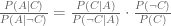
Their method is interesting. It’s called a case crossover design, and it works like this. We want to know the odds ratio of an accident when you talk on the phone versus when you don’t. Let’s write it like this, where 


But we have no way of estimating numerator or denominator from traffic accident data because we would need to know the counterfactuals of how often people drive (with and without talking on the phone) and don’t have accidents. Case crossover studies are based on a little algebraic trick which transforms the odds ratio into something we can estimate, with just a little more data. Using Bayes’ rule and two lines of algebra, we can rewrite it like this.
From accident data we can estimate the first term on the right-hand-side. We just calculate the fraction of accidents in which someone was talking on the phone. The finesse comes in when we estimate the second term. We don’t want to just estimate the overall frequency of cell phone use because we estimated the first term using a selected sample of people who had accidents. They may be different from the population as a whole. We want the cellphone usage rates for the people in our sample.
Case crossover studies take each person in the data who had an accident and ask them to report whether they were talking on the phone while driving at the same time of day one week before. Thus, each person generates their own control case. It’s a valid control because its the same person, driving at the same time, and on average therefore under the same conditions. These survey data are used to estimate the second term.
It’s really clever and its used a lot in epidemiological studies. (People get sick, some were exposed to some potential hazard, others not. The method is used to estimate the increase in risk of getting sick due to being exposed to the hazard.)
I have never seen it in economics however. In fact, this was the first I ever heard of it. So its natural to wonder why. And it doesn’t take long before you see that it has a serious weakness when applied to data with a lot of heterogeneity.
To see the problem, suppose that there are two types of people. The first group, in addition to being generally accident prone are also easily distracted. Everyone else is a safe driver and talking on cellphones doesn’t make them any less safe. Then our sample of people who actually had accidents would consist disproportionately of the first group. We would be estimating the effect of cell phone use on them alone. If they make up a small fraction of the population then we are drastically overestimating the increase in risk.
It’s fair to say that at best we can use the estimate of 4 as an upper bound on the risk ratio averaging over the entire population. That population average could be zero and still be consistent with the findings from case crossover studies. And there is no simple way to remedy the problems with this method. So I think there is good reason to approach this question from a different direction.
As I described before, if cell phone distractions increase accident risk we would see it by comparing the population of drivers to drivers with hearing impairment, who don’t use cell phones. And it turns out that the data exist. In the NHTSA’s database of traffic accidents, there is this variable:
P18 Person’s Physical Impairment
Definition: Identifies physical impairments for all drivers and non-motorists which may have contributed to the cause of the crash.
And “deaf” is impairment number 9.
