
You are currently browsing the tag archive for the ‘sport’ tag.
How does the additional length of a 5 set match help the stronger player? Commenters to my previous post point out the direct way: it lowers the chance of a fluke in which the weaker player wins with a streak of luck. But there’s another way and it can in principle be identified in data.
To illustrate the idea, take an extreme example. Suppose that the stronger player, in addition to having a greater baseline probability of winning each set, also has the ability to raise his game to a higher level. Suppose that he can do this once in the match and (here’s the extreme part) it guarantees that he will win that set. Finally, suppose that the additional effort is costly so other things equal he would like to avoid it. When will he use his freebie?
Somewhat surprisingly, he will always wait until the last set to use it. For example, in a three set match, suppose he loses the first set. He can spend his freebie in the second set but then he has to win the third set. If he waits until the third set, his odds of winning the match are exactly the same. Either way he needs to win one set at the baseline odds.
The advantage of waiting until the third set is that this allows him to avoid spending the effort in a losing cause. If he uses his freebie in the second set, he will have wasted the effort if he loses the third set. Since the odds of winning are independent of when he spends his effort, it is unambiguously better to wait as long as possible.
This strategy has the following implications which would show up in data.
- In a five set match, the score after three sets will not be the same (statistically) as the score in a three set match.
- In particular, in a five-set match the stronger player has a lower chance of winning a third set when the match is tied 1-1 than he would in a three set match.
- The odds that a higher seeded player wins a fifth set is higher than the odds that he wins, say, the second set. (This may be hard to identify because, conditional on the match going to 5 sets, it may reveal that the stronger player is not having a good day.)
- If the baseline probability is close to 50-50, then a 5 set match can actually lower the probability that the stronger player wins, compared to a 3 set match.
This “freebie” example is extreme but the general theme would always be in effect if stronger players have a greater ability to raise their level of play. That ability is an option which can be more flexibly exercised in a longer match.
- One implication of a theory I have written about before is that a best of 5 set match confers a greater advantage on the stronger player than a best of 3 set match. (The basic idea is that the 5 sets gives the stronger player more flexibility in timing his bursts of effort.) Here are some data that would shed light: compare men’s versus women’s Grand Slam matches in terms of the probability that a higher-seeded player will win. Even better: divide the data into non-Grand Slam and Grand Slam matches. Ask how much more likely a higher-seeded player wins a Grand Slam match versus a non-Grand Slam match. Do this for both women and men. Then do the difference-in-differences. This gives you a nice control because women play 3 sets whether its a Grand Slam or not. Men play 5 sets in Grand Slams and 3 sets in almost all non-Grand-Slam events.
- Four Grand Slams, only three surfaces. It’s time the US Open switched to ice. (with skates.)
I once wrote about height and speed in tennis arguing that negative correlation appears at the highest level simply because they are substitutes and the athletes are selected to be the very best. At the blog MickeyMouseModels.blogspot.com, there is a post which shows very nicely the effect using simulated data. Quoting:
Suppose that, in the general population, the distribution of height and speed looks roughly like this:
Where did I get this data? It’s entirely hypothetical. I made it up! That said, I did try to keep it semi-realistic: the heights are generated as H = 4 + U1 + U2 + U3 feet, where the U are independently uniform on (0, 1); the result is a bell curve on (4, 7) feet, which I prefer to the (-Inf, +Inf) of an actual normal distribution. (I’ve created something similar to the N=3 frame in this animation.)
The next step is to give individuals a maximum footspeed S = 10 + U4 + U5 + U6 mph, with the U independently uniform on (0, 5). By construction, speed is independent from height, and falls more or less in a bell curve from 10 to 25 mph. Fun anecdote: my population is too slow to include Usain Bolt, whose top footspeed is close to 28 mph.
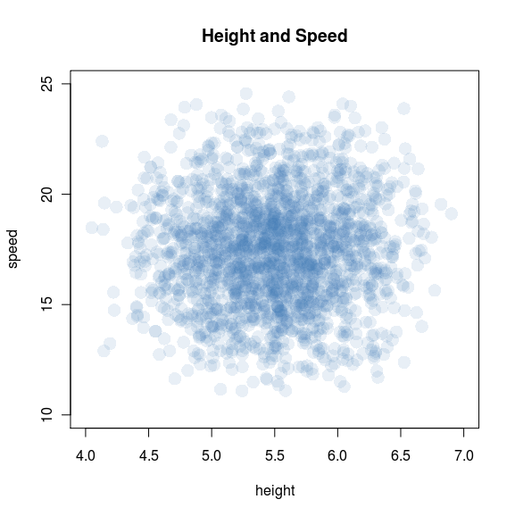
Back to tennis. Let’s imagine that tennis ability increases with both height and speed — and, moreover, that those two attributes are substitutable: if you’re short (and have a weak serve), you can make up for it by being fast. With that in mind, let’s revisit the scatterplot:
There it is: height and speed are independent in the general population, but very much dependent — and negatively correlated — among tennis players. The plot really drives the point home: top athletes will be either very tall, very fast, or nearly both; and excluding everyone else creates a downward slope.

Kobe Bryant was recently fined $100,000 for making a homophobic comment to a referee. Ryan O’Hanlon writing for The Good Men Project blog puts it into perspective:
- It’s half as bad as conducting improper pre-draft workouts.
- It’s twice as bad as saying you want to leave the NBA and go home.
- It’s just as bad as talking about the collective bargaining agreement.
- It’s twice as bad as saying one of your players used to smoke too much weed.
- It’s just as bad as writing a letter in Comic Sans about a former player.
- It’s just as bad as saying you want to sign the best player in the NBA.
- It’s four times as bad as throwing a towel to distract a guy when he’s shooting free throws.
- It’s four times as bad as kicking a water bottle.
- It’s 10 times as bad as standing in front of your bench for an extended period of time.
- It’s 10 times as bad as pretending to be shot by a guy who once brought a gun into a locker room.
- It’s 13.33 times as bad as tweeting during a game.
- It’s five times as bad as throwing a ball into the stands.
- It’s four times as bad as throwing a towel into the stands.
- It’s twice as bad as lying about smelling like weed and having women in a hotel room during the rookie orientation program.
- It’s one-fifth as bad as snowboarding.
That’s based on a comparison of the fines that the various misdeeds earned. The “n times as bad” is the natural interpretation of the fines since we are used to thinking of penalties as being chosen to fit the crime. But NBA justice needn’t conform to our usual intuitions because this is an employer/employee relationship governed by actual contract, not just social contract. We could try to think of these fines as part of the solution to a moral hazard problem. Independent of how “bad” the behaviors are, there are some that the NBA wants to discourage and fines are chosen in order to get the incentives right.
But that’s a problematic interpretation too. From the moral hazard perspective the optimal fine for many of these would be infinite. Any finite fine is essentially a license to behave badly as long as the player has a strong enough desire to do so. Strong enough to outweigh the cost of the fine. You can’t throw a towel to distract a guy when he’s shooting free throws unless its so important to you that you are willing to pay $250,000 for the privilege.
You can rescue moral hazard as an explanation in some cases because if there is imperfect monitoring then the optimal fine will have to be finite. Because with imperfect monitoring the fine cannot be a perfect deterrent. For example it may not possible to detect with certainty that you were lying about smelling like weed and having women in a hotel room during the rookie orientation program. If so then the false positives will have to be penalized. And when the fine will be paid with positive probability even with players on their best behavior you are now trading off incentives vs. risk exposure.
But the imperfect monitoring story can’t explain why Comic Sans doesn’t get an infinite fine, purifying the game of that transgression once and for all. Or tweeting, or snowboarding or most of the others as well.

It could be that the NBA knows that egregious fines can be contested in court or trigger some other labor dispute. This would effectively put a cap on fines at just the level where it is not worth the player’s time and effort to dispute it. But that doesn’t explain why the fines are not all pegged at that cap. It could be that the likelihood that a fine of a given magnitude survives such a challenge depends on the public perception of the crime . That could explain some of the differences but not many. Why is the fine for saying you want to leave the NBA larger than the fine for throwing a ball into the stands?
Once we’ve dispensed with those theories it just might be that the NBA recognizes that players simply want to behave badly sometimes. Without that outlet something else is going to give. Poor performance perhaps or just an eventual Dennis Rodman. The NBA understands that a fine is a price. And with the players having so many ways of acting out to choose from, the NBA can use relative prices to steer them to the efficient frontier. Instead of kicking a water bottle, why not get your frustrations out by sending 3 1/2 tweets during the game? Instead of saying that one of your players smokes too much weed, go ahead and indulge your urge to stand out in front of the bench for an extended period of time. You can do it for 5 times as long as the last guy or even stand 5 times farther out.
Not surprisingly, all of these choices start to look like real bargains compared to snowboarding and impoper pre-draft workouts.
Nonsense?
For Shmanske, it’s all about defining what counts as 100% effort. Let’s say “100%” is the maximum amount of effort that can be consistently sustained. With this benchmark, it’s obviously possible to give less than 100%. But it’s also possible to give more. All you have to do is put forth an effort that can only be sustained inconsistently, for short periods of time. In other words, you’re overclocking.
And in fact, based on the numbers, NBA players pull greater-than-100-percent off relatively frequently, putting forth more effort in short bursts than they can keep up over a longer period. And giving greater than 100% can reduce your ability to subsequently and consistently give 100%. You overdraw your account, and don’t have anything left.
Here is the underlying paper. <Painfully repressing the theorist’s impulse to redefine the domain to paths of effort rather than flow efforts, thus restoring the spiritually correct meaning of 100%>
Cap curl: Tim Carmody guest blogging at kottke.org.
In tennis, a server should win a larger percentage of second-serve points compared to first-serve points; that much we know. Partly that’s because a server optimally serves more faults (serves that land out) on first serve than second serve. But what if we condition on the event that the first serve goes in? Here’s a flawed logic that takes a bit of thinking to see through:
Even conditional on a first serve going in, the probability that the server wins the point must be no larger than the total win probability for second serves. Because suppose it were larger. Then the server wins with a higher probability when his first serve goes in. So he should ease off just a bit on his first serve so that a larger percentage lands in, raising the total probability that he wins the point. Even though the slightly slower first serve wins with a slightly reduced probability (conditional on going in) he still has a net gain as long as he eases off just slightly so that it is still larger than the second serve percentage. Indeed the lower probability of a fault could even raise the total probability that he wins on the first serve.

Seth Godin writes:
When two sides are negotiating over something that spoils forever if it doesn’t get shipped, there’s a straightforward way to increase the value of a settlement. Think of it as the net present value of a stream of football…
Any Sunday the NFL doesn’t play, the money is gone forever. You can’t make up for it later by selling more football–that money is gone. The owners don’t get it, the players don’t get it, the networks don’t get it, no one gets it.
The solution: While the lockout/strike/dispute is going on, keep playing. And put all the profit/pay in an escrow account. Week after week, the billions and billions of dollars pile up. The owners see it, the players see it, no one gets it until there’s a deal.
There are two questions you have to ask if you are going to evaluate this idea. First, what would happen if you change the rules in this way? Second, would the parties actually agree to it?
Bargaining theory is one of the most unsettled areas of game theory, but there is one very general and very robust principle. What drives the parties to agreement is the threat of burning surplus. Any time a settlement proposal on the table it comes with the following interpretation: “if you don’t agree to this now you better expect to be able to negotiate for a significantly larger share on the next round because between now and then a big chunk of the pie is going to disappear.” Moreover it is only through the willingness to let the pie shrink that either party can prove that he is prepared to make big sacrifices in order to get that larger share.
So while the escrow idea ensures that there will be plenty of surplus once they reach agreement, it has the paradoxical effect of making agreement even more difficult to reach. In the extreme it makes the timing of the agreement completely irrelevant. What’s the point of even negotiating today when we can just wait until tomorrow?
But of course who cares when and even whether they eventually agree? All we really want is to see football right? And even if they never agree how to split the mounting surplus, this protocol keeps the players on the field. True, but that’s why we have to ask whether the parties would actually accept this bargaining game. After all if we just wanted to force the players to play we wouldn’t have to get all cute with the rules of negotiation, we could just have an act of Congress.
And now we see why proposals like this can never really help because they just push the bargaining problem one step earlier, essentially just changing the terms of the negotiation without affecting the underlying incentives. As of today each party is looking ahead expecting some eventual payoff and some total surplus wasted. Godin’s rules of negotiation would mean that no surplus is wasted so that each party could expect an even higher eventual payoff. But if it were possible to get the two parties to agree to that then for exactly the same reason under the old-fashioned bargaining process there would be a proposal for immediate agreement with the same division of the spoils on the table today and inked tomorrow.
Still it is interesting from a theoretical point of view. It would make for a great game theory problem set to consider how different rules for dividing the accumulated profits would change the bargaining strategies. The mantra would be “Ricardian Equivalence.”
Jonah Lehrer writes about how bad NFL teams are at drafting talented players, particularly at the quarterback position.
Despite this advantage, however, sports teams are impressively amateurish when it comes to the science of human capital. Time and time again, they place huge bets on the wrong players. What makes these mistakes even more surprising is that teams have a big incentive to pick the right players, since a good QB (or pitcher or point guard) is often the difference between a middling team and a contender. (Not to mention, the player contracts are worth tens of millions of dollars.) In the ESPN article, I focus on quarterbacks, since the position is a perfect example of how teams make player selection errors when they focus on the wrong metrics of performance. And the reason teams do that is because they misunderstand the human mind.
He talks about a test that is given to college quarterbacks eligible for the NFL draft to test their ability to make good decisions on the field. Evidently this test is considered important by NFL scouts and indeed scores on this test are good predictors of whether and when a QB will be selected in the draft.
However,
Consider a recent study by economists David Berri and Rob Simmons. While they found that Wonderlic scores play a large role in determining when QBs are selected in the draft — the only equally important variables are height and the 40-yard dash — the metric proved all but useless in predicting performance. The only correlation the researchers could find suggested that higher Wonderlic scores actually led to slightly worse QB performance, at least during rookie years. In other words, intelligence (or, rather, measured intelligence), which has long been viewed as a prerequisite for playing QB, would seem to be a disadvantage for some guys. Although it’s true that signal-callers must grapple with staggering amounts of complexity, they don’t make sense of questions on an intelligence test the same way they make sense of the football field. The Wonderlic measures a specific kind of thought process, but the best QBs can’t think like that in the pocket. There isn’t time.
I have not read the Berri-Simmons paper but inferences like this raise alarm bells. For comparison, consider the following observation. Among NBA basketball players, height is a poor predictor of whether a player will be an All-Star. Therefore, height does not matter for success in basketball.
The problem is that, both in the case of IQ tests for QBs and height for NBA players, we are measuring performance conditional on being good enough to compete with the very best. We don’t have the data to compare the QBs who are drafted to the QBs who are not and how their IQ factors into the difference in performance.
The observable characteristic (IQ scores, height) is just one of many important characteristics, some of which are not quantifiable in data. Given that the player is selected into the elite, if his observable score is low we can infer that his unobservable scores must be very high to compensate. But if we omit those intangibles in the analysis, it will look like people with low scores are about as good as people with high scores and we would mistakenly conclude that they don’t matter.

I am always writing about athletics from the strategic point of view: focusing on the tradeoffs. One tradeoff in sports that lends itself to strategic analysis is effort vs performance. When do you spend the effort to raise your level of play and rise to the occasion?
My posts on those subjects attract a lot of skeptics. They doubt that professional athletes do anything less than giving 100% effort. And if they are always giving 100% effort, then the outcome of a contest is just determined by gourd-given talent and random factors. Game theory would have nothing to say.
We can settle this debate. I can think of a number of smoking guns to be found in data that would prove that, even at the highest levels, athletes vary their level of performance to conserve effort; sometimes trying hard and sometimes trying less hard.
Here is a simple model that would generate empirical predictions. Its a model of a race. The contestants continuously adjust how much effort to spend to run, swim, bike, etc. to the finish line. They want to maximize their chance of winning the race, but they also want to spend as little effort as necessary. So far, straightforward. But here is the key ingredient in the model: the contestants are looking forward when they race.
What that means is at any moment in the race, the strategic situation is different for the guy who is currently leading compared to the trailers. The trailer can see how much ground he needs to make up but the leader can’t see the size of his lead.
If my skeptics are right and the racers are always exerting maximal effort, then there will be no systematic difference in a given racer’s time when he is in the lead versus when he is trailing. Any differences would be due only to random factors like the racing conditions, what he had for breakfast that day, etc.
But if racers are trading off effort and performance, then we would have some simple implications that, if it were born out in data, would reject the skeptics’ hypothesis. The most basic prediction follows from the fact that the trailer will adjust his effort according to the information he has that the leader does not have. The trailer will speed up when he is close and he will slack off when he has no chance.
In terms of data the simplest implication is that the variance of times for a racer when he is trailing will be greater than when he is in the lead. And more sophisticated predictions would follow. For example the speed of a trailer would vary systematically with the size of the gap while the speed of a leader would not.
The results from time trials (isolated performance where the only thing that matters is time) would be different from results in head-to-head competitions. The results in sequenced competitions, like downhill skiing, would vary depending on whether the racer went first (in ignorance of the times to beat) or last.
And here’s my favorite: swimming races are unique because there is a brief moment when the leader gets to see the competition: at the turn. This would mean that there would be a systematic difference in effort spent on the return lap compared to the first lap, and this would vary depending on whether the swimmer is leading or trailing and with the size of the lead.
And all of that would be different for freestyle races compared to backstroke (where the leader can see behind him.)
Finally, it might even be possible to formulate a structural model of an effort/performance race and estimate it with data. (I am still on a quest to find an empirically oriented co-author who will take my ideas seriously enough to partner with me on a project like this.)
Drawing: Because Its There from www.f1me.net
It is within the letter of the law of NHL hockey to employ a goalie who is obese enough to sit on the ice and obstruct the entire mouth of the goal. But can you get away with it?
As strange as it may sound to anyone with a sense of decency, there is actually sound reasoning behind it. Because of the geometry of the game, the potential for one mammoth individual to change hockey is staggering. Simply put, there is a goal that’s 6 feet wide and 4 feet high, and a hockey puck that needs to go into it in order to score. Fill that net completely, and no goals can possibly be scored against your team. So why hasn’t it happened yet?
One answer is that professionalism and fair play prevent many sports teams from doing whatever it takes to win. This is also known as “having no imagination.” Additionally, in hockey the worry of on-ice reprisal from bloodthirsty goons would weigh heavily on the mind of any player whose very existence violated the game’s “unwritten rules.”
Hit the link for the full analysis, including a field experiment. In a WSJ excerpt from a book entitled Andy Roddick Beat Me With A Frying Pan. Helmet huck: Arthur Robson.
Boston being a center for academia as well as professional sports, Harvard and MIT faculty and students are leading the way in the business of sports consulting.
And some of those involved aren’t that far away from being kids. Harvard sophomore John Ezekowitz, who is 20, works for the NBA’sPhoenix Suns from his Cambridge dorm room, looking beyond traditional basketball statistics like points, rebounds, assists, and field goal percentage to better quantify player performance. He is enjoying the kind of early exposure to professional sports once reserved for athletic phenoms and once rare at institutions like Harvard and MIT. “If I do a good job, I can have some new insight into how this team plays, what works and what doesn’t,” says Ezekowitz. “To think that I might have some measure of influence, however small, over how a team plays is a thrill.” It’s not a bad job, either. While he doesn’t want to reveal how much he earns as a consultant, he says that not only does he eat better than most college students, the extra cash also allows him to feed his golf-club-buying habit.
Almost every kind of race works like this: we agree on a distance and we see who can complete that distance in the shortest time. But that is not the only way to test who is the fastest. The most obvious alternative is to switch the roles of the two variables: fix a time and see who can go the farthest in that span of time.
Once you think of that the next question to ask is, does it matter? That is, if the purpose of the race is to generate a ranking of the contestants (first place, second place, etc) then are there rankings that can be generated using a fixed-time race that cannot be replicated using an appropriately chosen fixed-distance race?
I thought about this and here is a simple way to formalize the question. Below I have represented three racers. A racer is characterized by a curve which shows for every distance how long it takes him to complete that distance.

Now a race can be represented in the same diagram. For example, a standard fixed-distance race looks like this.

The vertical line indicates the distance and we can see that Green completes that distance in the shortest time, followed by Black and then Blue. So this race generates the ranking Green>Black>Blue. A fixed-time race looks like a horizontal line:

To determine the ranking generated by a fixed-time race we move from right to left along the horizontal line. In this time span, Black runs the farthest followed by Green and then Blue.
(You may wonder if we can use the same curve for a fixed-time race. After all, if the racers are trying to go as far as possible in a given length of time they would adjust their strategies accordingly. But in fact the exact same curve applies. To see this suppose that Blue finishes a d-distance race in t seconds. Then d must be the farthest he can run in t seconds. Because if he could run any farther than d, then it would follow that he can complete d in less time than t seconds. This is known as duality by the people who love to use the word duality.)
OK, now we ask the question. Take an arbitrary fixed-time race, i.e. a horizontal line, and the ordering it generates. Can we find a fixed-distance race, i.e. a vertical line that generates the same ordering? And it is easy to see that, with 3 racers, this is always possible. Look at this picture:

To find the fixed-distance race that would generate the same ordering as a given fixed-time race, we go to the racer who would take second place (here that is Black) and we find the distance he completes in our fixed-time race. A race to complete that distance in the shortest time will generate exactly the same ordering of the contestants. This is illustrated for a specific race in the diagram but it is easy to see that this method always works.
However, it turns out that these two varieties of races are no longer equivalent once we have more than 3 racers. For example, suppose we add the Red racer below.

And consider the fixed-time race shown by the horizontal line in the picture. This race generates the ordering Black>Green>Blue>Red. If you study the picture you will see that it is impossible to generate that ordering by any vertical line. Indeed, at any distance where Blue comes out ahead of Red, the Green racer will be the overall winner.
Likewise, the ordering Green>Black>Red>Blue which is generated by the fixed-distance race in the picture cannot be generated by any fixed-time race.
So, what does this mean?
- The choice of race format is not innocuous. The possible outcomes of the race are partially predetermined what would appear to be just arbitrary units of measurement. (Indeed I would be a world class sprinter if not for the blind adherence to fixed-distance racing.)
- There are even more types of races to consider. For example, consider a ray (or any curve) drawn from the origin. That defines a race if we order the racers by the first point they cross the curve from below. One way to interpret such a race is that there is a pace car on the track with the racers and a racer is eliminated as soon as he is passed by the pace car. If you play around with it you will see that these races can also generate new orderings that cannot be duplicated. (We may need an assumption here because duality by itself may not be enough, I don’t know.)
- That raises a question which is possibly even a publishable research project: What is a minimal set of races that spans all possible races? That is, find a minimal set of races such that if there is any group of contestants and any race (inside or outside the minimal set) that generates some ordering of those contestants then there is a race in the set which generates the same ordering.
- There are of course contests that are time based rather than quantity based. For example, hot dog eating contests. So another question is, if you have to pick a format, then which kinds of feats better lend themselves to quantity competition and which to duration competition?
It occurs to me that in our taxonomy of varieties of public goods, we are missing a category. Normally we distinguish public goods according to whether they are rival/non-rival and whether they are excludable/non-excludable. It is generally easier to efficiently finance excludable public goods because people by the threat of exclusion you can get users to reveal how much they are willing to pay for access to the public good.
I read this article about Piracy of sports broadcasts and I started to wonder what effect it will have on the business of sports. Free availability of otherwise exclusive broadcasts mean that professional sports change from an excludable to a non-excludable public good. This happened to software and music but unique aspects of those goods enable alternative revenue sources (support in the case of software, live performance in the case of music.)
For sports the main alternative is advertising. And the only way to ensure that the ads can’t be stripped out of the hijacked broadcast, we are going to see more and more ads directly projected onto the players and the field.
And then I started wondering what would be the analogue of advertising to support other non-excludable public goods. The key property is that you cannot consume the good without being exposed to the ad. What about clean air? National defense?
But then I realized that there is something different about these public goods. Not only are they not excludable– a user cannot be prevented from using it, but they are not avoidable — the user himself cannot escape the public good. And there is no reason to finance unavoidable public goods by any means other than taxation.
Here’s the point. If the public good is avoidable, you can increase the user tax (by bundling ads) and trust that those who don’t value the public good very much will stop using it. Given the level of the tax it would be inefficient for them to use it. Knowing that this inefficiency can be avoided you have more flexibility to raise the tax, effectively price discriminating high-value users.
If the public good is unavoidable, everyone pays whether you use ads or just taxation (uncoupled with usage), so there really isn’t any difference.
So this category of an avoidable public good seems a useful one. Can you think of other examples of non-excludable but avoidable public goods? Sunsets: avoidable. National defense: unavoidable.
Here’s a broad class of games that captures a typical form of competition. You and a rival simultaneously choose how much effort to spend and depending on your choices, you earn a score, a continuous variable. The score is increasing in your effort and decreasing in your rival’s effort. Your payoff is increasing in your score and decreasing in your effort. Your rival’s payoff is decreasing in your score and his effort.
In football, this could model an individual play where the score is the number of yards gained. A model like this gives qualitatively different predictions when the payoff is a smooth function of the score versus when there are jumps in the payoff function. For example, suppose that it is 3rd down and 5 yards to go. Then the payoff increases gradually in the number of yards you gain but then jumps up discretely if you can gain at least 5 yards giving you a first down. Your rival’s payoff exhibits a jump down at that point.
If it is 3rd down and 20 then that payoff jump requires a much higher score. This is the easy case to analyze because the jump is too remote to play a significant role in strategy. The solution will be characterized by a local optimality condition. Your effort is chosen to equate the marginal cost of effort to the marginal increase in score, given your rival’s effort. Your rival solves an analogous problem. This yields an equilibrium score strictly less than 20. (A richer, and more realistic model would have randomness in the score.) In this equilibrium it is possible for you to increase your score, even possibly to 20, but the cost of doing so in terms of increased effort is too large to be profitable.
Suppose that in the above equilibrium you gain 4 yards. Then when it is 3rd down and 5 this equilibrium will unravel. The reason is that although the local optimality condition still holds, you now have a profitable global deviation, namely putting in enough effort to gain 5 yards. That deviation was possible before but unprofitable because 5 yards wasn’t worth much more than 4. Now it is.
Of course it will not be an equilibrium for you to gain 5 yards because then your opponent can increase effort and reduce the score below 5 again. If so, then you are wasting the extra effort and you will reduce it back to the old value. But then so will he, etc. Now equilibrium requires mixing.
Finally, suppose it is 3rd down and inches. Then we are back to a case where we don’t need mixing. Because no matter how much effort your opponent uses you cannot be deterred from putting in enough effort to gain those inches.
The pattern of predictions is thus: randomness in your strategy is non-monotonic in the number of yards needed for a first down. With a few yards to go strategy is predictable, with a moderate number of yards to go there is maximal randomness, and then with many yards to go, strategy is predictable again. Variance in the number of yards gained in these cases will exhibit a similar non-monotonicity.
This could be tested using football data, with run vs. pass mix being a proxy for randomness in strategy.
While we are on the subject, here is my Super Bowl tweet.
I am talking about world records of course. Tyler Cowen linked to this Boston Globe piece about the declining rate at which world records are broken in athletic events, especially Track and Field. (Usain Bolt is the exception.)
How quickly should we expect the rate of new world records to decline? Suppose that long jumps are independent draws from a Normal distribution. Very quickly the world record will be in the tail. At that point breaking the record becomes very improbable. But should the rate decline quickly from there? Two forces are at work.
First, every new record pushes us further into the tail and reduces the probability, and hence freqeuncy, of new records. But, because of the thin tail property of the Normal distribution, new records will with very high probability be tiny advances. So the new record will be harder to beat but not by very much.
So the rate will decline and asymptotically it will be zero, but how fast will it converge to zero? Will there be a constant K such that we will have to wait no more than nK years for the nth record to be broken or will it be faster than that?
I am sure there is an easy answer to this question for the Normal distribution and probably a more general result, but my intuition isn’t taking me very far. Probably this is a standard homework problem in probability or statistics.
The Boston Globe piece is about humans ceasing to progress physically. The theory could shed light on this conclusion. If the answer above is that the arrival rate increases exponentially, I wonder what rate the mean of the distribution can grow and still give rise to the slowdown. If the mean grows logarithmically?
After winning her Australian Open semi-final match against Caroline Wozniacki, Li Na was interviewed on the court. She got some laughs when she complained that she was not feeling her best because her husband’s snoring had been keeping her up the night before. Then she was asked about her motivation.
Interviewer: What got you through that third set despite not sleeping well last night?
Li Na: Prize money.

Tennis commentators will typically say about a tall player like John Isner or Marin Cilic that their height is a disadvantage because it makes them slow around the court. Tall players don’t move as well and they are not as speedy.
On the other hand, every year in my daughter’s soccer league the fastest and most skilled player is also among the tallest. And most NBA players of Isner’s height have no trouble keeping up with the rest of the league. Indeed many are faster and more agile than Isner. LeBron James is 6’8″.
It is not true that being tall makes you slow. Agility scales just fine with height and it’s a reasonable assumption that agility and height are independently distributed in the population. Nevertheless it is true in practice that all of the tallest tennis players on the tour are slower around the court.
But all of these facts are easily reconcilable. In the tennis production function, speed and height are substitutes. If you are tall you have an advantage in serving and this can compensate for lower than average speed if you are unlucky enough to have gotten a bad draw on that dimension. So if we rank players in terms of some overall measure of effectiveness and plot the (height, speed) combinations that produce a fixed level of effectiveness, those indifference curves slope downward.
When you are selecting the best players from a large population, the top players will be clustered around the indifference curve corresponding to “ridiculously good.” And so when you plot the (height, speed) bundles they represent, you will have something resembling a downward sloping curve. The taller ones will be slower than the average ridiculously good tennis player.
On the other hand, when you are drawing from the pool of Greater Winnetka Second Graders with the only screening being “do their parent cherish the hour per week of peace and quiet at home while some other parent chases them around?” you will plot an amorphous cloud. The best player will be the one farthest to the northeast, i.e. tallest and fastest.
Finally, when the sport in question is one in which you are utterly ineffective unless you are within 6 inches of the statistical upper bound in height, then a) within that range height differences matter much less in terms of effectiveness so that height is less a substitute for speed at the margin and b) the height distribution is so compressed that tradeoffs (which surely are there) are less stark. Mugsy Bogues notwithstanding.

In a paper published in the Journal of Quantitative Analysis in Sports; Larsen, Price, and Wolfers demonstrate a profitable betting strategy based on the slight statistical advantage of teams whose racial composition matches that of the referees.
We find that in games where the majority of the officials are white, betting on the team expected to have more minutes played by white players always leads to more than a 50% chance of beating the spread. The probability of beating the spread increases as the racial gap between the two teams widens such that, in games with three white referees, a team whose fraction of minutes played by white players is more than 30 percentage points greater than their opponent will beat the spread 57% of the time.
The methodology of the paper leaves some lingering doubt however because the analysis is retrospective and only some of the tested strategies wind up being profitable. A more convincing way to do a study like this is to first make a public announcement that you are doing a test and, using the method discussed in the comments here, secretly document what the test is. Then implement the betting strategy and announce the results, revealing the secret announcement.
In sports, high-powered incentives separate the clutch performers from the chokers. At least that’s the usual narrative but can we really measure clutch performance? There’s always a missing counterfactual. We say that he chokes if he doesn’t come through when the stakes are raised. But how do we know that he wouldnt have failed just as miserably under normal circumstances? As long as performance has a random element, pure luck (good or bad) can appear as if it were caused by circumstances.
You could try a controlled experiment, and probably psychologists have. But there is the usual leap of faith required to extrapolate from experimental subjects in artificial environments to professionals trained and selected for high-stakes performance.
Here is a simple quasi-experiment that could be done with readily available data. In basketball when a team accumulates more than 5 fouls, each additional foul sends the opponent to the free-throw line. This is called the “bonus.” In college basketball the bonus has two levels. After fouls 5-10 (correction: fouls 7-9) the penalty is what’s called a “one and one.” One free-throw is awarded, and then a second free-throw is awarded only if the first one is good. After 10 fouls the team enters the “double bonus” where the shooter is awarded two shots no matter what happens on the first. (In the NBA there is no “single bonus,” after 5 fouls the penalty is two shots.)
The “front end” of the one-and-one is a higher stakes shot because the gain from making it is 1+p points where p is the probability of making the second. By contrast the gain from making the first of two free throws is just 1 point. On all other dimensions these are perfectly equivalent scenarios, and it is the most highly controlled scenario in basketball.
The clutch performance hypothesis would imply that success rates on the front end of a one and one are larger than success rates on the first free-throw out of two. The choke-under-pressure hypothesis would imply the opposite. It would be very interesting to see the data.
And if there was a difference, the next thing to do would be to analyze video to look for differences in how players approach these shots. For example I would bet that there is a measurable difference in the time spent preparing for the shot. If so, then in the case of choking the player is “overthinking” and in the clutch case this would provide support for an effort-performance tradeoff.
One way players might play a game is by learning over time till they reach a best response to strategies they have observed in the past. If learning converges, then a natural hypothesis due to Fudenberg and Levine , is that it settles on a self-confirming equilibrium:
Self-Confirming Equilibrium (SCE) is a relaxation of Nash equilibrium: Each player chooses a best response to his beliefs and his beliefs are “correct” on the path of play. But different players may have different beliefs over strategies off the path of play and may believe that players’ actions are correlated. Nash equilibrium (NE) requires that players’ beliefs are also correct off the path of play, that all players have the same beliefs over off the path play and that players’ strategies are independent. As the definition of Nash equilibrium puts extra constraints on beliefs, the set of Nash equilibria of a game cannot be larger than the set of self-confirming equilibria.
There is no reason why learning based on past play should tell us anything about off path play. So SCE is a more natural prediction for the outcome of learning than NE. Finally, we come to college football!
The University of Oregon football team has been pursuing an innovative “off the path” strategy:
“Oregon plays so fast that it is not uncommon for it to snap the ball 7 seconds into the 40-second play clock, long before defenses are accustomed to being set. That is so quick that opponents have no ability to substitute between plays, and fans at home do not have time to run to the fridge.”
Opposing teams on defense are just not used to playing against this strategy and have not developed a best-response. So far they have come up with an import from soccer, the old fake an injury strategy. This has yielded great moments like the YouTube video above.
I am trying to relate this football scenario to SCE. SCE does not incorporate experimentation which is what the Oregon Ducks are trying so this is immediately inconsistent with SCE. But set that aside – even without experimentation, is the status quo of slower snaps and best responses to them an SCE? I think it is and that it is even consistent with NE.
Even in a SCE of the two player sequential move game of football, the offense has to hypothesize what the defense would do if the offense plays fast. Given their conjecture about the defense’s play if the offense plays fast, it is better for the offense to play slow rather than play fast. Their conjecture about the defense’s play to fast snaps does not have to be at a best response for the defense as this node is unreached. And the defense plays a best response to what they observe – slow play by the offense. So both players are at a best response and the offense’s conjecture about the defense play off the path of play can be taken to be “correct” as neither SCE nor NE put restrictions on the defense being at a best response off the path of play.
In other words, in two player games, a SCE is automatically a NE. From diagonalizing Fudenberg and Levine, it seems this that this is true if you rule out correlated strategies (but I am administering an exam as I write this so I cannot concentrate!). If I am right, the football example is consistent with SCE and hence NE. (In three (or more) player games, there can be a substantive difference between SCE and NE as different players can have different conjectures on off path play in SCE but not NE and this can turn out to be important.)
But the football experience is not necessarily a Subgame Perfect Equilibrium. This adds the requirement of sequential rationality to Nash equilibrium: Each player’s strategy at all decision nodes, even those off the path of play, has to be a best response to his beliefs and beliefs have to be correct etc. So, it may be that football teams on offense have been assuming there is some devastating loss to playing fast. First, it is simply hard to play fast and perhaps they thought it was easy to defend fast snaps. But since this was never really tested, no-one really knew it for a fact.
Now the Oregon Ducks are experimenting and their opponents are trying to find a best response. So far they have come up with faking injuries. Eventually they will find a best response. Then and only then will the teams learn whether it is better for the offense to have fast snaps or slow snaps. And then they will play subgame perfect equilibrium: the offense may switch back to slow snaps if the best response to fast snaps if sufficiently devastating.
Today Qatar was the surprise winner in the bid to host the FIFA World Cup in 2022, beating Japan, The United States, Australia, and Korea. It’s an interesting procedure by which the host is decided consisting of multiple rounds of elimination voting. 22 judges cast ballots in a first round. If no bidder wins a majority of votes then the country with the fewest votes is eliminated and a second round of voting commences. Voting continues in this way for as many rounds as it takes to produce a majority winner. (It’s not clear to me what happens if there is a tie in the final round.)
Every voting system has its own weaknesses, but this one is especially problematic giving strong incentives for strategic voting. Think about how you would vote in an early round when it is unlikely that a majority will be secured. Then, if it matters at all, your vote determines who will be eliminated, not who will win. If you are confident that your preferred site will survive the first round, then you should not vote truthfully. Instead you should to keep bids alive that will easier to beat in later rounds.
Can we look at the voting data and identify strategic voting? As a simple test we could look at revealed preference violations. For example, if Japan survives round one and a voter switches his vote from Japan to another bidder in round two, then we know that he is voting against his preference in either round one or two.
But that bundles together two distinct types of strategic voting, one more benign than the other. For if Japan garners only a few votes in the first round but survives, then a true Japan supporter might strategically abandon Japan as a viable candidate and start voting, honestly, for her second choice. Indeed, that is what seems to have happened after round one. Here are the data.

We have only vote totals so we can spot strategic voting only if the switches result in a net loss of votes for a surviving candidate. This happened to Japan but probably for the reasons given above.
The more suspicious switch is the loss of one vote for the round one leader Qatar. One possibility is that a Qatar supporter , seeing Qatar’s survival to round three secured, cast a strategic vote in round two to choose among the other survivors. But the more likely scenario in my opinion is a strategic vote for Qatar in round one by a voter who, upon learning from the round 1 votes that Qatar was in fact a contender, switched back to voting honestly.
We focused our analysis on twelve distinct types of touch that occurred when two or more players were in the midst of celebrating a positive play that helped their team (e.g., making a shot). These celebratory touches included fist bumps, high fives, chest bumps, leaping shoulder bumps, chest punches, head slaps, head grabs, low fives, high tens, full hugs, half hugs, and team huddles. On average, a player touched other teammates (M = 1.80, SD = 2.05) for a little less than two seconds during the game, or about one tenth of a second for every minute played.
That is the highlight from the paper “Tactile Communication, Cooperation, and Performance” which documents the connection between touching and success in the NBA. Controlling (I can’t vouch for how well) for variables like salary, preseason expectations, and early season success, the conclusion is: the more hugs in the first half of the season the more success in the second half.
The data on first vs. second serve win frequency cannot be taken at face value because of selection problems that bias against second serves. The general idea is that first serves always happen but second serves happen only when first serves miss. The fact that the first serve missed is information that at this moment serving is harder than usual. In practice this can be true for a number of reasons: windy conditions, it is late in the match, or the server is just having a bad streak. In light of this, we can’t conclude from the raw data that professional tennis players are using sub-optimal strategy on second serves.
To get a better comparison we need an identification strategy: some random condition that determines whether the next serve will be a first or second serve. We would restrict our data set to those random selections. Sounds hopeless?
When a first serve hits the net and goes in it is a “let” and the next serve is again a first serve. But if it goes out then it is a fault. The impact with the net introduces the desired randomness, especially when the ball hits the tape and bounces up. Conditional on hitting the tape, whether it lands in or out can be considered statistically independent of the server’s current mental state, the wind conditions, and the stage of the game. These are the ingredients for a “natural experiment.”
Here is Sandeep’s post on the data discussed in the New York Times about winning percentages on first and second serves in tennis.There are a few players who win with higher frequency on either the first or second serve and this is a puzzle. Daniel Khaneman even gets drawn into it. (To be precise, we are calculating the probability she wins on the first serve and comparing that to the probability she wins conditional on getting to her second serve. At least that is the relevant comparison, this is not made clear in the article. Also I agree with Sandeep that the opponent must be taken into consideration but there is a lot we can say about the individual decision problem. See also Eilon Solan.)
And the question persists: would players have a better chance of winning the point, even after factoring in the sure rise in double faults, by going for it again on the second serve — in essence, hitting two first serves?
But this is the wrong way of phrasing the question and in fact by theory alone, without any data (and definitely no psychology), we can prove that most players do not want to hit two first serves.
One thing is crystal clear, your second serve should be your very best. To formalize this, let’s model the variety of serves in a given player’s arsenal. For our purposes it is enough to describe a serve by two numbers. Let 


Your second serve should be the one that has the highest
But it’s a jumped-to conclusion that this means your second serve should be as good as your first serve. Because your first serve should typically be worse!
On your first serve it’s not just
So, you want in your arsenal a serve which has a lower
But at the margin, if you can reduce
So when Vanderbilt tennis coach Bill Tym says
“It’s an insidious disease of backing off the second serve after they miss the first serve,” said Tym, who thinks that players should simply make a tiny adjustment in their serves after missing rather than perform an alternate service motion meant mostly to get the ball in play. “They are at the mercy of their own making.”
he might be just thinking about it backwards. The second serve is their best serve, but nevertheless it is a “backing-off” from their first serve because their first serve is (intentionally) excessively risky.
Statistically, the implications of this strategy are
- The winning percentage on first serves should be lower than on second serves.
- First serves go in less often than second serves.
- Conditional on a serve going in, the winning percentage on the first serve should be higher than on second serves.
The second and third are certainly true in practice. And these refute the idea that the second serve should use the same technique as the first serve as suggested by the Vanderbilt coach. The first is true for most servers sampled in the NY Times piece.
In golf:
How big a deal is luck on the golf course? On average, tournament winners are the beneficiaries of 9.6 strokes of good luck. Tiger Woods’ superior putting, you’ll recall, gives him a three-stroke advantage per tournament. Good luck is potentially three times more important. When Connolly and Rendleman looked at the tournament results, they found that (with extremely few exceptions) the top 20 finishers benefitted from some degree of luck. They played better than predicted. So, in order for a golfer to win, he has to both play well and get lucky.
I don’t understand the statistics enough to evaluate this paper. Apparently they call “luck” the residual in some estimate of “skill.” What I don’t understand is how such luck can be distinguished from unexpectedly good performance. If a schlub wins a big tournament and then returns to being a schlub, is that automatically luck?
I wrote previously about the equilibrium effects of avoiding spoilers. You might want to strategically generate spoilers to counteract these effects. I just discovered that a website exists for generating spoilers: shouldiwatch.com.
The premise is that you have recorded a sporting event on your DVR and you want to enjoy watching it. Enjoyment has something to do with the resolution of uncertainty. So you have preferences for the time path of uncertainty resolution. Maybe you want your good news in lumps and your bad news revealed gradually. Maybe you like suspense. A mechanism can fine tune and enhance these.
But it always cuts two ways. A spoiler creates a discrete jump in your beliefs at the beginning followed by another effect on your beliefs as the game unfolds. For example, ShouldIWatch.com allows me to set a program that will warn me when the Lakers beat the Celtics by more than 10 points. The idea is that I don’t want to watch a blowout. But there is an effect on my beliefs: knowing that it is not a blowout changes my expectations at the beginning of the game. Then there is a second effect during the game: if the Lakers take a 15 point lead, I am expecting a come-back by the Celtics. In return for the increased excitement at the beginning I pay with reduced excitement in the interim.
This trade-off could make for a cool model. An event will unfold over time. An observer cares about the outcome and cares about the path of his beliefs but will watch the event after it is over. A mechanism is a program which knows the full path of the event and reveals information to the observer before and while he watches the event. Design the mechanism which maximizes the observer’s overall expected value taking into account this tradeoff.
File this under psychological mechanism design.
- Are civil wars more often North vs South than East vs West? Put differently, based on the boundaries that have survived until today, are countries, on average, wider than they are tall?
- Which will arrive first: the ability to make a digital “mold” of distinctive celebrity voices or the technology allowing celebrities to map the digital signature of their voice in order to claim property rights?
- The hard `r` in Spanish and other languages creates a natural syncopation because the r usually occupies the downbeat, as in “sagrada” or “cortado”
- Syncopation adds a dimension to music because brain tickles as it tries to make sense of two times at once.
- Among European soccer nations, the closer to Africa the fewer black players on the national team.

If you play tennis then you know the coordination problem. Fumbling in your pocket to grab a ball and your rallying partner doing the same and then the kabuki dance of who’s gonna pocket the ball and who’s going to hit first? Sometimes you coordinate, but seemingly just as often the balls are simultaneously repocketed or they cross each other at the net after you both hit.
Rallying with an odd number of balls gives you a simple coordination device. You will always start with an unequal number of balls, and it will always be common knowledge how many each has even if the balls are in your pockets.
I used to think that the person holding 2 or more should hit first. That’s a bad convention because after the first rally you are back to a position of symmetry. (And a convention based on who started with two will fail the common knowledge test due to imperfect memory, especially when the rally was a long one.)
Instead, the person holding 1 ball should hit first. Then the subgame following that first rally is trivially solved because there is only one feasible convention.
By the way, this observation is a key lemma in any solution to Tyler Cowen’s tennis ball problem.
Of course this works with any odd number of balls. But five is worse. It becomes too hard to keep track of so many balls and eventually you will lose common knowledge of the total number of balls in rotation.
It gets harder and harder to avoid learning the outcome of a sporting event before you are able to get home and watch it on your DVR. You have to stop surfing news web sites, stay away from Twitter, and be careful which blogs you read. Even then there is no guarantee. Last year I stopped to get a sandwich on the way home to watch a classic Roddick-Federer Wimbledon final (16-14 in the fifth set!) and some soccer-moms mercilessly tossed off a spoiler as an intermezzo between complaints about their nannys.
No matter how hard you try to avoid them, the really spectacular outcomes are going to find you. The thing is, once you notice that you realize that even the lack of a spoiler is a spoiler. If the news doesn’t get to you, then at the margin that makes it more likely that the outcome was not a surprise.
Right now I am watching Serena Williams vs Yet-Another-Anonymous-Eastern-European and YAAEE is up a break in the first set. But I am still almost certain that Serena Williams will win because if she didn’t I probably would have found out about it already.
This is not necessarily a bad thing. Unless the home team is playing, a big part of the interest in sports is the resolution of uncertainty. We value surprise. Moving my prior further in the direction of certainty has at least one benefit: In the event of an upset I am even more surprised. This has to be taken into account when I decide the optimal amount of effort to spend trying to avoid spoilers. It means that I should spend a little less effort than I would if I was ignoring this compensating effect.
It also tells me something about how to spend that effort. I once had a match spoiled by the Huffington Post. I never expected to see sports news there, but ex post I should have known that if HP is going to report anything about tennis it is going to be when there was an upset. You won’t see “Federer wins again” there.
Finally, if you really want to keep your prior and you recognize the effects above, then there is one way to generate a countervailing effect. Have your wife watch first and commit to a random disclosure policy. Whenever the favorite won, then with probability p she informs you and with probability 1-p she reveals nothing.
FIFA experimented with a “sudden-death” overtime format during the 1998 and 2002 World Cup tournaments, but the so-called golden goal was abandoned as of 2006. The old format is again in use in the current World Cup, in which a tie after the first 90 minutes is followed by an entire 30 minutes of extra time.
One of the cited reasons for reverting to the old system was that the golden goal made teams conservative. They were presumed to fear that attacking play would leave them exposed to a fatal counterattack. But this analysis is questionable. Without the golden goal attacking play also leaves a team exposed to the possibility of a nearly-insurmountable 1 goal deficit. So the cost of attacking is nearly the same, and without the golden goal the benefit of attacking is obviously reduced.
Here is where some simple modeling can shed some light. Suppose that we divide extra time into two periods. Our team can either play cautiously or attack. In the last period, if the game is tied, our team will win with probability 

Then, assigning a value of 1 for a win and -1 for a loss, 
Now we are in the first period of extra time. Here’s how we will model the tradeoff between attacking and playing cautiously. If we attack, we increase by 

If we don’t attack there is some probability of a goal scored, and some probability of a scoreless first period. So what we are really doing by attacking is taking an
In the golden goal system, the event of a scoreless first period leads to value
.
(A chunk of sized 

This inequality is comparing the value of the event of a scoreless first period
Rearranging, we attack if
.
Now, if we switch to the current system, a goal in the first period is not decisive. Let’s write
Now the comparison is changed because attacking only alters probability-chunks of sized 

,
which re-arranges to

and since 

The golden goal encourages attacking play. The intuition coming from the formulas is the following. If 

And if 


I haven’t checked it but I would guess that the conclusion is the same for any number of “periods” of extra time (so that we can think of a period as just representing a short interval of time.)
